ICCAS 2005 June 2-5, KINTEX, Gyeonggi-Do, Korea
Training an Artificial Neural Network
for Estimating the Power Flow State
Alireza Sedaghati
Faculty of Electrical Engineering and Robotics, Shahrood University of Technology
(E-mail:
[email protected]
)
Abstract: The principal context of this research is the approach to an artificial neural network algorithm which solves multivariable
nonlinear equation systems by estimating the state of line power flow. First a dynamical neural network with feedback is used to find the minimum value of the objective function at each iteration of the state estimator algorithm. In second step a two-layer neural network structures is derived to implement all of the different matrix-vector products that arise in neural network state estimator analysis. For hardware requirements, as they relate to the total number of internal connections, the architecture developed here preserves in its structure the pronounced sparsity of power networks for which state the estimator analysis is to be carried out. A principal feature of the architecture is that the computing time overheads in solution are independent of the dimensions or structure of the equation system. It is here where the ultrahigh-speed of massively parallel computing in neural networks can offer major practical benefit.
Keywords: Power flow; State estimator; Neural network
1. INTRODUCTION
Of the numerous different application are as of neural networks that have been developed or proposed previously, those related to numerical analysis appear to be mainly in optimization in which scalar objective function is to minimized [1–4]. The neural network architectures proposed for linear or nonlinear optimization with or without constraints include. Hopfield type networks [1] and layered networks with feedbacks, which implement the steepest descent algorithm [2–4].
The principal aim of the development in numerical analysis methods which this paper seeks to report is that of deriving a neural network which implements the state estimator algorithm [5] for solving multivariable nonlinear equation systems. When implemented in hardware, the architecture achieves ultrahigh-speed computation. Individual multiplications in all of the matrix vector product operations, which arise implemented in parallel. A principal feature of the architecture is that the computing time overheads in solution are independent of the dimensions or structure of the equation system, which is solved.
The main step in being able to exploit the parallel processing which neural networks offer is that of solving, as a minimization problem, the linearized equation system to which state estimator method [5] leads at each iteration. Dynamic neural network with feedback provide means of implementing this form of unconstraint function minimization. The main context of the research reported is that of state estimator analysis in a power system. Whilst the computing overheads in analysis are nowadays unlikely to be at issue, there is scope for further advances in on-line forms of
power flow measurements in digital computer control and monitoring for power system.
The main steps of the research reported here are:
(a) Using a dynamical neural network with feedback to find the minimum value of the objective function at each ’the state estimator algorithm’ iteration.
(b) Deriving two-layer neural network structures to implement all of the different matrix-vector products that arise in neural network state estimator analysis.
2. THE LINE POWER FLOW
STATE ESTIMATOR
The instrumentation around the bus can be divided into injections, bus metering, and line flow measurements. Each of the measurements monitors all three phases in order to calculate positive sequence values. The following assumptions are made:
1. balanced three-phase flow conditions are present, and the system is in steady-state operation,
2. accuracy of metering is known (i.e. the meter reading are accurate to 1%, 2%, etc. of the true physical value), 3. the full-scale range of each meter is known (e.g. 0–100MW,
0–50MVar, etc.).
The errors in converting the analog quantities to digital signals for the data link to the central computer are known 0.25% error, 0.1% error, and so on due to discrimination. Each measurement of line flow in any remote terminal unit, in complex form:
(1) has a specified weighting factor inversely proportional to its accuracy.
(2) In Eq. (2), c is the accuracy expressed as a decimal of the 1
real and reactive flow, typically 0.01 or 0.02, c2 is the
transducer and analog-to-digital converter accuracy in decimal form, typically 0.0025, 0.005 and FS is the full-scale range of both the MW and MVar readings.
The factor 50×10-6 is selected to normalize subsequent
numerical quantities. The absolute value of the measurement is used in the denominator, so the weighting factor Wi is
recomputed each time a new measurement is made.
The weighted-least-squares state estimator is to find the best state vectors X, which minimizes the performance index of M measurements, J:
(3) where Smi is a power flow measurement and Sci is a
calculated value based on the state X. The power flow calculated at bus i is
(4) The measured numerical values Smi are equated flow from
bus voltages to be calculated:
(5) The power flow measurement depends primarily on the difference in voltage from bus i to bus k, so the equivalent measured differences are:
(6) Rewriting Eq. (6) in matrix form yields:
(7) where H is an M*M diagonal matrix, K is a vector, and EM is
vector of measured differences associated with each power flow measurement. Even though the bus voltages on the right hand side of Eq. (7) are unknown, E , can be considered to M
be derived from SM. A matrix formulation of the state
estimator performance index is
(8) where SM is an M vector of the measurements, W is a
diagonal weighting matrix, and S is the calculated power C
flow vector. In Eq. (8) substitute the measurement vector, Eq. (7) and a calculated power flow:
(9) Substituting Eq. (9) into Eq. (8) yields:
(10)
The calculated voltage difference vector can be expressed in terms of the bus voltages, EBUS, and the slack voltage Er:
(11) In Eq. (11), A is a double branch to bus incidence matrix, in other words, 1 and 1 in each row, corresponding to a measurement along a directed branch element. When line flows are measured on each end, the series element appears twice. The order of A is M*N, where N is the number of buses, A is partitioned into a bus voltage part, B, and a slack bus vector b.
(12)
Substituting Eq. (11) into Eq. (10) yields:
(13) The product H*WH is assumed to be constant [5] and Eq. (13) is minimized with respect to the bus voltage vector:
(14)
Either of the conjugate forms may be used to solve for EBUS
in order to minimize the performance index:
(15) Let D = H*WH, a diagonal matrix of order M, and the iterative line flow state estimator is
(16)
where k +1 is the next iteration, and k M
E is evaluated using the previous value of EBUS. The algorithm to solve for the bus
voltage vector in the state estimator is (1) Guess an initial k
BUS
E . A flat start sets all bus voltages equal to the slack bus.
(2) Use the measurement data to calculate the initial voltage difference:
where both H and K depend on k BUS
E .
(3) Minimize J with respect to the bus voltage vector, k BUS
E and find k+1
BUS
E .
(4) Repeat steps 2 and 3 until convergence to within a desired error tolerance. The tolerance is usually expressed in terms of change in bus voltages between iterations:
(5) If the result of the last equation is okey, stop the iteration, otherwise use k → k + 1 and go to step 2.
Observe that the approximation of constant H*WH = D does not affect the accuracy of converged results. The matrix D appears as an approximation to a gradient multiplication on the right-hand side of Eq. (15).
3. DYNAMICAL GRADIENT SYSTEM
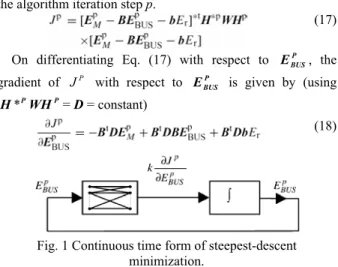
Using J for the objective function (8) to be minimized at P
the algorithm iteration step p.
(17) On differentiating Eq. (17) with respect to P
BUS
E , the
gradient of J with respect to P P BUS E is given by (using P PWH H * = D = constant) (18)
Fig. 1 Continuous time form of steepest-descent minimization.
Conventional iterative algorithms for minimizing a scalar objective function J have their basis in solving for the P
necessary condition in which the gradient vector ∂J/∂ P BUS
E is
equal to zero at the minimum point. In the steepest-descent algorithm:
(19) In Eq. (19), n identifies the iteration step of the steepestdescent minimization procedure. Scalar coefficient η is
often referred to as the ‘step length’ of the method. On rearranging Eq. (19):
(20) Starting from an initial condition P
BUS
E (0), Eq. (20) provides a
means, by which the value P BUS
ICCAS 2005 June 2-5, KINTEX, Gyeonggi-Do, Korea
at the each iteration until convergence:
(21) Eq. (20) has the form of a difference equation in which n can be interpreted as a discrete time step counter. On that basis, P
BUS
E (n)- P
BUS
E (n-1) provides a finite difference
approximation to the first order derivative of P BUS
E with
respect to time. Interpreting the derivative in this way in the continuous time domain, leads to the following first order differential equation of the steepest-descent algorithm:
(22) In the Eq. (22), k is a negative scalar constant. An outline is
shown in Fig. 1 of a dynamic neural based on feedbacks, which solves the differential equation system of Eq. (22). The evaluation of the gradient vector ∂J /∂P P
BUS
E of Eq. (18) is achieved by means of a neural network like ref. [6].
4. MATRIX VECTOR PRODUCTS IN
NEURAL NETWORKS
Each of the several matrix vector products involved in forming the gradient vector ∂J /∂P P
BUS
E is implemented in two-layer feed forward networks in which the processing function for each node is a linear one. The combination of networks required to form the gradient vector ∂J /∂P P
BUS
E is
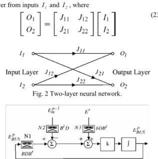
best derived by via the Eqs. (18) and (22). It can be formed Fig. 2. The network in Fig. 2 forms O1 and O2 in the output
layer from inputs I1 and I2, where
(23)
Fig. 2 Two-layer neural network.
Fig. 3 Design of neural network for finding the state estimator correction vector P
BUS
E
The weights of the cross-connections between input and output layer nodes correspond in value to the off diagonal element of the matrix. The pattern of cross-connections in the network derives directly from the nonzero off diagonal element pattern in the matrix. The combination of networks required to form the gradient vector ∂J /∂P P
BUS
E is best
derived by breaking down the task into four distinct parts. Working from the extreme right-hand side of Eq. (18), the first matrix-vector product term to be evaluated is P
BUS
E [BtDB].
Inputs to nodes in the input layer of a two layer neutral network of the form in Fig. 3 are elements of vector P
BUS
E [BtDB] matrix is convenient to identify this neural network by N1 in Fig. 3.
Finally, integrating the gradient vector multiplied by k gives the P
BUS
E (n). The closed loop in Fig. 3 formed by
feeding P BUS
E (n) back into the input layer of neural network
N1 settles to a value for which the quadratic function J is P
zero.
Fig. 4 gives the digital or discrete time form of the array of neural network of Fig. 3. The time delay operator in the steepest descent minimization is denoted by z and the time -1
step identifier by n. As in Eq. (20), the correction vector at nth. Steepest-descent step is formed in Fig. 4 from
(24)
Fig. 4 A numerical form of neural network architecture for the state estimator algorithm.
Fig. 5 A part of the neural network for the power flow state estimator algorithm.
The time n is incremented in successive passes of the
principal loop in Fig. 4 until a convergence criterion is full-filled. Convergence of the loop in the discrete form of Fig. 4 corresponds to the dynamic feedback loop in the continuous time system of Fig. 3 setting to a steady solution. The term of
1 -P m
E seen in Fig. 4 is not measurement matrix obtained directly from an energy system therefore Smi must be used
instead of P-1 m
E with the help of Eqs. (6) and (7). The overall neural network for the state estimator algorithm is shown in Fig. 5. The global feedback loop relates to the state estimator algorithm in which the step counter p is incremented at the
each iteration. The local feedback loop is that of the steepest descent minimization of quadratic function J at each the P
state estimator iteration. It can be obtained the overall the neural network state estimator algorithm in Fig. 6 by substituting Fig. 5 into Fig. 4. The term of F in Fig. 6 is a shift operator advances the solution from one state estimator iteration step to the next. After stopping the whole algorithm,
P BUS
E is used to calculate ‘the best estimate’ for line flows by using Eq. (5). If the convergence is obtained at pth. iteration,
the best estimate for line flows will be (flowing from i to k
bus).
(25)
P
J is minimized at each the state estimator iteration,
checking for convergence in the loop is based on the criterion: (26) (27) Through the global feedback loop of Fig. 6, the overall the state estimator solution is advanced through successive the state estimator given in ref. [5] iterations to convergence. Checking the convergence of this loop is based on:
(28) (29)
Fig. 6 The neural network state estimator algorithm. For a sparse power network where there are few branches connected to each power network node, the structure of neural networks N1, N2, N3 is also sparse one. There are few connections to each neural network node.
5. OBTAINING THE NEURAL NETWORKS
Let us assume that real and reactive line flows are measured at both ends of three transmission lines on the power transmission system with three-bus and three-line in Fig. 7. The set of power flow measurements, using a Sbase MVA
floating voltage base are Sm12, Sm21, Sm13, Sm31, Sm23 and m32
S . Z31, Z23 and Z12 are complex impedances of the lines.
The subscripts ik of Smik are shown the direction of power
flow measurement from bus i to bus k. The line charging and
shunt terms are negligible. Consider each line flow measurement to perform with c1 accurate meters with Sbase1
MVA, Sbase2 MVar full-scale (FS) range, and c2 transducer
errors. The weighting factor for measurement from bus i and
bus k computed using Eq. (2) is
(30)
Fig. 7 The three-bus system.
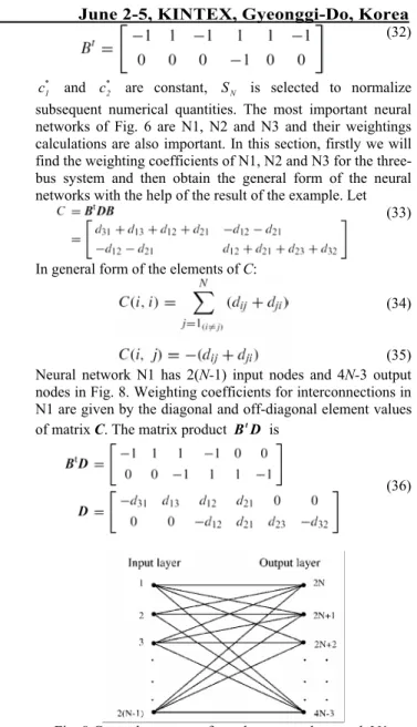
All voltages be 1.0 in the product H*WH, so the diagonal weighting matrix is (31) (32) * 1 c and * 2
c are constant, S is selected to normalize N
subsequent numerical quantities. The most important neural networks of Fig. 6 are N1, N2 and N3 and their weightings calculations are also important. In this section, firstly we will find the weighting coefficients of N1, N2 and N3 for the three-bus system and then obtain the general form of the neural networks with the help of the result of the example. Let
(33)
In general form of the elements of C:
(34) (35) Neural network N1 has 2(N-1) input nodes and 4N-3 output
nodes in Fig. 8. Weighting coefficients for interconnections in N1 are given by the diagonal and off-diagonal element values of matrix C. The matrix product BtD is
(36)
Fig. 8 General structure of two-layer neural network N1.
If a measurement is at the near end of a line connected to bus i, dm is positive, and negative for a measurement at the
far end of a line to this bus. Assume that P M t P BDE X = and using Eq. (36): (37) Neural network N2 has 2M input nodes and 2(N-1) output
nodes. The matrix product bDB is t
Fig. 9 Overall neural networks for the power flow state estimator.
ICCAS 2005 June 2-5, KINTEX, Gyeonggi-Do, Korea
(38)
Assume that Q = r
t
bDB E and using Eq. (38)
(39)
Neural network N3 has two input nodes and 2(N-1) output
nodes. Let us assume that
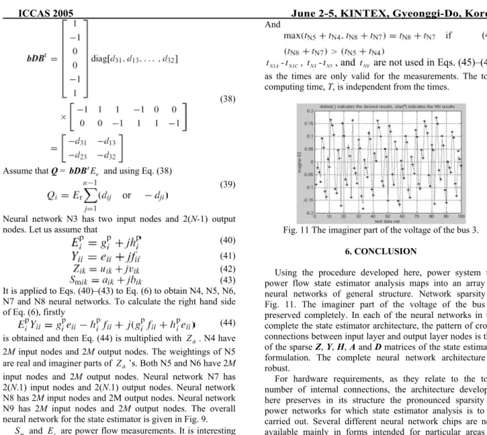
(40) (41) (42) (43) It is applied to Eqs. (40)–(43) to Eq. (6) to obtain N4, N5, N6, N7 and N8 neural networks. To calculate the right hand side of Eq. (6), firstly
(44) is obtained and then Eq. (44) is multiplied with Zik. N4 have
2M input nodes and 2M output nodes. The weightings of N5
are real and imaginer parts of Zik’s. Both N5 and N6 have 2M
input nodes and 2M output nodes. Neural network N7 has
2(N.1) input nodes and 2(N.1) output nodes. Neural network
N8 has 2M input nodes and 2M output nodes. Neural network
N9 has 2M input nodes and 2M output nodes. The overall
neural network for the state estimator is given in Fig. 9.
m
S and Er are power flow measurements. It is interesting
to quantify the total computation time of the neural system of Fig. 9. For this purpose, NG is used for the total number of the state estimator iterations and tN1-tN9 are used for the
computation times in solution in neural networks N1–N9, respectively. If NL(p) is the number of iterations in the local
loop which minimizes quadratic function J at each state P
estimator step and T is the total computing time of the
complete architecture of Fig. 9.
(45)
In Eq. (45)
(46)
Fig. 10. The real part of the voltage of the bus 3
And
(47)
N1C N1A-t
t , tN3-tN5
, and
tN9are not used in Eqs. (45)–(47)
as the times are only valid for the measurements. The total computing time, T, is independent from the times.
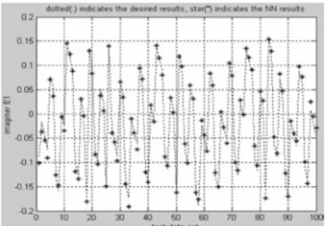
Fig. 11 The imaginer part of the voltage of the bus 3.
6. CONCLUSION
Using the procedure developed here, power system the power flow state estimator analysis maps into an array of neural networks of general structure. Network sparsity is Fig. 11. The imaginer part of the voltage of the bus 3. preserved completely. In each of the neural networks in the complete the state estimator architecture, the pattern of cross-connections between input layer and output layer nodes is that of the sparse Z, Y, H, A and D matrices of the state estimator formulation. The complete neural network architecture is robust.
For hardware requirements, as they relate to the total number of internal connections, the architecture developed here preserves in its structure the pronounced sparsity of power networks for which state estimator analysis is to be carried out. Several different neural network chips are now available mainly in forms intended for particular areas of application. More general systems now at an advanced stage of development have recently been reported [7].
Fig. 12 The real part of the voltage of the bus 1. The principal context of the research reported here is that of real time control in integrated power network system with particular reference to the SCADA functions. It is here where the ultrahigh-speed of massively parallel computing in neural networks can offer major practical benefit.
7. THE RESULTS OF THE SAMPLE SYSTEM
AND THE EVALUATIONS
In this paper, the three-bus and three-line power transmission system shown in Fig. 7 is considered and studied. The line impedance values of the sample system, using 100MVA
floating voltage base are given in Table 1. An each line-flow measurement is performed with c1= 0.02 or 2% accurate
meters with 100MW, 100MVar full-scale range, and c2=
0.005 transducer errors.
Fig. 13 The imaginer part of the voltage of the bus 1. Table 1
It is purposed to realize by using a multi-layer feed-forward NN architecture the estimation of the bus voltages without measuring at some buses where it is difficult to measure the active and reactive powers in the power systems in this paper.
Fig. 14 The real part of the voltage of the bus 2.
Fig. 15 The imaginer part of the voltage of the bus 2. The two-layer neural network (NN) structure is trained for data set of the number of one thousand by changing the amplitude of bus 3 (slack bus) in the range (0.9 pu) and (1.1 pu) and the angle of bus 3 in the range of (.10.) and (10.) as random. The NN structure is trained by using the Levenberg– Marquardt algorithm. After training, the performance of the NN is shown by applying the test data set of the number of one hundred. While this data set is made up, the active and reactive powers of the buses 2 and 3 are applied as the NN inputs and the real and imaginer parts of the voltages of the buses 1, 2 and 3 are obtained as the NN outputs.
Consequently, the NN structure has eight inputs (i.e. the active and reactive parts of S12, S21, S13 and S23), six outputs (i.e. the real and imaginer Fig. 15. The imaginer part of the voltage of the bus 2. parts of E1, E2 and E3), one hidden layer, and 32
neurons in the hidden layer. Thus, it is shown that E1, E2, and E3 values are estimated without measuring the active and
reactive power of bus 3 (slack bus) and the measurement is saved.
As it is shown in Figs. 10–15, the estimation performance of the NN for the real parts of the bus voltages is nearly perfect and the estimation performance of the NN for the imaginer parts of the bus voltages is fairly well. Our ongoing researches in the next stage are the power flow state estimator analysis of the large power systems and integrated ac–dc power systems via the more different multi-layer NN architecture. In near future, it is studied to make up for a different paper by our.
REFERENCES
[1] D.W. Tank, J.J. Hopfield, Simple “neural” optimization networks: an A/D converter, signal decision circuit, and a linear programming circuit, IEEE Trans. CAS-33 (5) (1986) 533–541.
[2] M.P. Kennedy, L.O. Chua, Neural networks for nonlinear programming, IEEE Trans. CAS-35 (5) (1988) 554–562. [3] V.A. Rodriguez, et al., Non-linear switched capacitor neural networks for optimisation problems, IEEE Trans. CAS-37 (3) (1990) 384–398.
[4] C.Y. Maa, M.A. Shanblatt, Linear and quadratic programming neural network analysis, IEEE Trans. NN-3 (4) (1992) 580–594.
[5] G.L. Kusic, Computer-Aided Power Systems Analysis, Prentice-Hall, NJ, USA, 1986.
[6] T.T. Nguyen, Neural network load flow, IEE Proc. Gener. Transm. Distrib. 142 (1) (1995) 51–58.
[7] T. Watanabe, et al., A single 1.5-V digital chip for a 106 synapse neural network, IEEE Trans. NN-4 (3) (1993) 387– 393.