ICCAS2005 June 2-5, KINTEX, Gyeonggi-Do, Korea
Least-squares Lattice Laguerre Smoother
Dong Kyoo Kim∗and PooGyeon Park∗∗∗Electrical And Electronic Engineering Pohang Univ. Of Sci. and Tech., Pohang, KYUNGBUK 790-784 SOUTH KOREA (phone: +82-54-279-5588, fax: +82-54-279-2903; Email:kdk@postech.ac.kr)
∗∗Electrical And Electronic Engineering Pohang Univ. Of Sci. and Tech., Pohang, KYUNGBUK 790-784 SOUTH KOREA (phone: +82-54-279-2238, fax: +82-54-279-2903; Email:ppg@postech.ac.kr)
Abstract: This paper introduces the least-squares order-recursive lattice (LSORL) Laguerre smoother that has order-recursive smoothing structure based on the Laguerre signal representation. The LSORL Laguerre smoother gives excellent performance for a channel equalization problem with smaller order of tap-weights than its counterpart algorithm based on the transversal filter structure. Simulation results show that the LSORL Laguerre smoother gives better performance than the LSORL transversal smoother.
Keywords: Laguerre filter, smoother, least-squares estimation, adaptive filters 1 Introduction
Scattering channels, including wireless indoor channels, acoustic room channels, and damped-long impulse response systems, have significant multipath problem which leads to lots of efforts for characterizing such channels [1]. Almost measurements of scattering channels show that the chan-nels have long and oscillatory channel impulse responses. In case of wireless data communications, a receiver should employ a channel equalization to eliminate interferences be-tween adjacent symbols transmitted through the channels from a transmitter. Especially, it is well-known that non-causal channel equalization by delaying signals is required to consider the pre-cursor interference as well as the post-cursor, which requires smoothing, rather than filtering, for the channel equalization. The LSORL transversal smoother, which has some advantages such as computational efficiency, stage-to-stage modularity, and numerical robustness, was in-troduced in [2]. However, the transversal structure is inade-quate for the channel equalization because it requires plenty of filter-tap orders to equalize such channels. The Laguerre sequences are excellent for characterizing long and lowpass-filtered oscillatory impulse responses [3], thus this character-istics is suitable for the scattering channel equalization. Re-cently, [3] proposed an RLS Laguerre prediction algorithm having the lattice structure. By extending the work, this pa-per introduces the LSORL Laguerre smoother that is suit-able for equalizing above-mentioned channels.
2 Main results
Laguerre sequence is known as Li(z, a) , √1 − a2(z−1−
a)i(1 − az−1)−(i+1) = L
0(z, a)Ai(z, a), where A(z, a) ,
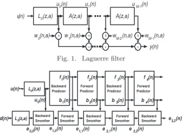
(z−1− a)(1 − az−1)−1. As in Figure 1, the Laguerre filter
output is written as yM(n, a) =PM −1i=0 wi(n, a)ui(n, a). We
shall obtain the least-squares order-recursive lattice Laguerre smoother by exploiting data structure that comes from the Laguerre filter proposed in [3]. For convenience, we shall henceforth fix the scale parameter a as a certain value; how to determine the best “a” is beyond scope of this paper. The least-squares cost function for M (, p + f )-th order
smooth-ing error is defined as
JMf (n) , e H p,f(n)ep,f(n), ep,f(n) , df(n) − HM(n)wp,f(n), where df(n) , [df(0) · · · df(n)]T, wp.f(n) , [w0(n) · · · wM −1(n)]T,
and HM(n) is a data matrix defined in (3). Then, the two
(M + 1)-th order forward and backward smoothing errors [4] are
ep,f +1(n) = df +1(n) − HM+1(n)wp,f +1(n), (1)
ep+1,f(n) = df(n) − HM+1(n)wp+1,f(n). (2)
The difference of the two smoothing errors is that they use different desired vectors and thus different weight vectors. To obtain the order-update recursion for the forward smoothing error (1), we partition the (M + 1)-th order data matrix as
HM +1(n) = u0(0) u1(0) · · · uM(0) .. . ... . .. ... u0(n) u1(n) · · · uM(n) = [u0(n) ¯HM(n)]. (3)
The optimal estimate of the desired vector, ˆdf +1(n), can be
written as ˆ
dp,f +1(n) = HM +1(n)(HM +1(n)HM +1(n))H −1·
HM +1(n)dH f +1(n). (4)
Using the above data matrix partition, the inverse of
HH M +1(n)HM +1(n) , RM +1(n) is written as R−1 M +1(n) = " 0 0T 0 R¯−1 M(n) # + 1 ξfM(n) " 1 − ˆwfM(n) # h 1 − ˆwMf H(n) i , (5) where ˆwf M(n) satisfies ¯ RM(n) ˆwfM(n) = H¯ H M(n)u0(n), ξf M(n) = f H M(n)fM(n), fM(n) = u0(n) − ¯HM(n) ˆwfM(n). 1189
If we substitute (5) for R−1
M +1 in (4), we get the following
recursion ˆ dp,f +1(n) = H¯M(n) ˆ¯wp,f +1(n) +fMH(n)df +1(n)ξ−fM(n)fM(n), ˆ¯ wp,f +1(n) = R¯−1M(n) ¯H H M(n)df +1(n).
Thus, we get an order-update recursion for the forward smoothing error,
ep,f +1(n) = ¯ep,f +1(n) − fMH(n)df +1(n)ξ−fM(n)fM(n), (6)
where ¯ep,f +1(n) = df +1(n) − ¯HM(n) ˆw¯p,f +1(n). Now, we
shall explain the relation between ep,f +1(n) and ¯ep,f(n).
Using the following lower triangular Toeplitz matrix as sug-gested in [3], Φ(n) = −a 1 − a2 −a .. . . .. . .. an−1(1 − a2) · · · 1 − a2 −a ,
it holds that ¯HM(n) = Φ(n)HM(n), and df +1(n) =
Φ(n)df(n). With these relations, we can write
ˆ¯ wp,f +1(n) = ³ HHM(n)ΦH(n)Φ(n)HM(n) ´−1 · HH M(n)ΦH(n)Φ(n)df +1(n). (7)
We use the following relation, ΦH(n)Φ(n) = I − c(n)cH(n),
where c(n) ,√1 − a2£an an−1 · · · a 1¤T
. If we put the relation into (7), we can get a useful equation,
¯ ep,f +1(n) = Φ(n)ep,f(n) + Φ(n)ˆcM(n)ζM−c(n)c H (n)ep,f(n), (8) where ˆcM(n) = HM(n)R−1 M(n)HMH(n)c(n), and ζMc (n) = 1 − cH(n)ˆc
M(n). The last element of ¯ep,f +1(n) can be simply
rewritten shown at 9-th line in Table 2.1., where φ(n) =
a−1√1 − a2cH(n) + [0 0 · · · − 1/a], and ˜cM(n) = c(n) −
ˆ
cM(n),. In the sequel, we have obtained two recursions for
the forward smoothing error as shown in Table 2.1.. Similarly
to the forward smoothing error, the order-update recursion for the backward smoothing error (2) is obtained as
ep+1,f(n) = ep,f(n) − bHM(n)df +1(n)ξ−bM(n)bM(n), (9)
where bM(n) is the backward prediction error and ξMb (n) =
bH
M(n)bM(n). Now, we need a time-update recursion for
cH(n)e
p,f(n)(, χM(n)) in (8), which is easily obtained by
using the time-update relation of cross-correlation of two er-ror vectors as appeared in [5],
χM(n) = aχM(n − 1) + ˜c∗M(n)γM−1(n)ep,f(n). (10)
where γM(n) is the well-known conversion factor. Using the
proposed order-recursive Laguerre prediction algorithm [3], the LSORL Laguerre smoother was obtained as shown in Table 2.1., where the prediction part is omited in this paper by the page limit.
L0(z,a) y(n) u0(n) A(z,a) A(z,a) X w0(n,a) w X 1(n,a) + X + X + wM-2(n,a) wM-1(n,a) u(n) u1(n) uM-1(n)
Fig. 1. Laguerre filter
Backward Predictor Forward Predictor Backward Predictor Forward Predictor Forward Smoother Backward Smoother Forward Smoother Backward Smoother L0(z,a) u(n) d(n) L0(z,a) Backward Smoother u0(n) e0,0(n) f1(n) b1(n) f2(n) f3(n) f4(n) b2(n) b3(n) b4(n) e1,0(n) e1,1(n) e2,1(n) e2,2(n) e3,2(n)
Fig. 2. The LSORL Laguerre smoother 2.1. Numerical examples and conclusion
Bernoulli sequence with ±1 is generated and fed into an IIR-typed channel with
H(z) =(0.866z
−1− 0.866z−2+ 0.2165z−3
(1 + 0.3z−1+ 0.3z−2+ 0.5z−3)−1
and the SNR at the channel output is set to 30dB. The lattice realization of the smoother is chosen as so-called ’BBFBF...’ form mentioned as shown in Figure 2; ’B’ stands for the backward smoothing and ’F’ stands for the forward smooth-ing. The tap-order of the LSORL Laguerre smoother is set to 6, and a is set to 0.5, which is obtained from a method proposed in [6]. For comparison, the 6-th order transver-sal LSORL smoother is used. Their MSE learning curves, which are averaged for 500 experiments, are depicted in Fig-ure 3. This figFig-ure shows that the LSORL Laguerre smoother outperforms the transversal LSORL smoother for the equal-ization of scattering channels.
In this paper, we introduced the LSORL Laguerre smoother. For equalizing a channel having a long and oscillatory impulse response, it showed better performance than its transversal counterpart.
References
[1] A.A.M. Saleh, and R. A. Valenzuela, “A statistical
model for indoor multipath propagation,” IEEE Journ.
Select. Areas Comm., Vol.5, No. 2, pp. 128-137, Feb.
1987. 0 50 100 150 200 250 300 350 400 450 500 10−4 10−3 10−2 10−1 100 iteration MSE
LSORL Transverasl smoother
LSORL Laguerre smoother
Fig. 3. Learning curves
Table 1. The LSORL Laguerre smoother For n=0,.... σm(−1) = ϕm(−1) = χm(−1) = 0 for all m e0,0(n) = ae0,0(n) + p 1 − a2d(n) For m=1,...,M-1
LSORL Laguerre prediction: Omitted. [3] LSORL Laguerre smoothing:
If m is odd, σM(n) = σM(n − 1) + ¯e∗p,f(n)¯γM−1(n)fM(n) ¯ ep,f +1(n) = −(ep,f(n) + χM(n)ζM−c(n)˜cM(n))/a ep,f +1(n) = ¯ep,f +1− σ∗ M(n)ξ−fM(n)fM(n) If m is odd, ϕM(n) = ϕM(n − 1) + e∗ p,f(n)γM−1(n)bM(n) ep+1,f(n) = ep,f(n) − ϕ∗M(n)ξ−bM(n)bM(n)
[2] J.T. Yuan and J.A. Stuller, “Least squares
order-recursive lattice smoothers,” IEEE Trans. Signal
Pro-cessing, vol. 43, pp. 1058-1067, 1995.
[3] R. Merched, and A. H. Sayed, “Order-recursive RLS
Laguerre adaptive filtering,” IEEE Trans. Signal
Pro-cessing, vol. 48, no. 11, pp. 3000-3010, Nov. 2000.
[4] D. K. Kim, and P. G. Park, “The normalized
least-squares order-recursive lattice smoother,” Signal
Pro-cessing, vol. 82, issue 6, pp. 895-905, June 2002.
[5] S. Haykin, Adaptive Filter Theory, 3rd ed., Englewood
Cliffs, NJ:Prentice-Hall, 1996.
[6] A.C. den Brinker, and B.E. Sarroukh, “Pole
optimisa-tion in adaptive Laguerre filtering ,” Proc. IEEE Int.
Conf. ICASSP-2004, vol. 2 , pp. 17-21, pp. II:649-652,
May 2004.