Neural Network Control Technique for Automatic Four Wheel Steered Highway Snowplow Robotic Vehicles

1. INTRODUCTION

Recently, researches on automation of highway maintenance and construction vehicles have been quite actively conducted. Fusing robotic technology to utility vehicles yields a new concept of robotic vehicles such as a crack sealing vehicle, trash pick up vehicle, and an autonomous corn-handling vehicle[1,2]. Several vehicles have been already commercialized.

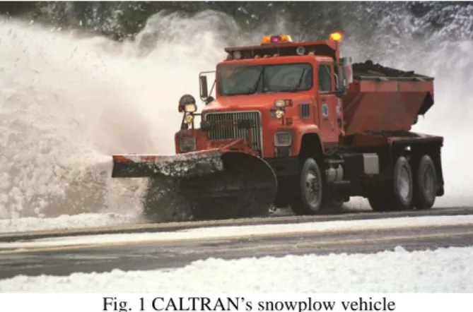
The advanced highway maintenance and construction technology (AHMCT) center at UC Davis has been known to be one of the leading research groups of conducting researches on this subject. One of their current projects is to automate and develop the snowplow vehicles. Snowplow vehicles are heavily used in mountain areas of having heavy snows in the winter. One typical snowplow vehicle is shown in Fig.1. To fully automate this kind of vehicle, automatic steering control should be developed along with GPS localization, GIS analysis, and sensor implementation.

The ultimate goal is to develop the snowplowing vehicle that can autonomously follow the guardrail of the highway without collision. The vehicle has to overcome the situation where the guardrail is hidden under the pile of snow. This requires accurate lateral control of the vehicle by maintaining a desired constant distance from the guardrail.

There have been many researches about lateral control of the vehicles.

H

_∞control and yaw rate feedback control methods for lateral positioning system have been proposed [3-5]. Experimental studies of robust lateral control of highway vehicles have also been conducted [6,7].

In our previous researches, neural network control technique has been applied for two wheel steering control of the bicycle model of the vehicle. Neural network with PD controllers has performed well to compensate for uncertainties. However, under the condition of heavy piles of snow, the front wheel steering may not be efficient. The rear steering control is also required for the better lateral control by helping the vehicle to push against snow. Many researches have been also considered the four wheeled drive vehicles. Fuzzy control methods have been used for steering four wheeled vehicles [8,9].

Fig. 1 CALTRAN’s snowplow vehicle

In this paper, as an extension of our previous researches, the neural network control technique is applied to a four wheeled drive bicycle model of the vehicle. The LQR control method is used to obtain optimal controller gains. Even though the LQR controller can stabilize the system and works quite well, tracking performance under snowplowing load becomes very poor. A neural network controller is introduced to compensate for uncertainties. Neural network has been known as a powerful nonlinear controller and used intensively in the area of robot and motion control applications [9,10]. Recently, successful real time neural network applications have been achieved [11-14].

Simulation studies have been conducted and position tracking performances are compared with those of the LQR controller under the virtual plowing condition.

2. FOUR WHEEL DRIVE VEHICLE DYNAMICS

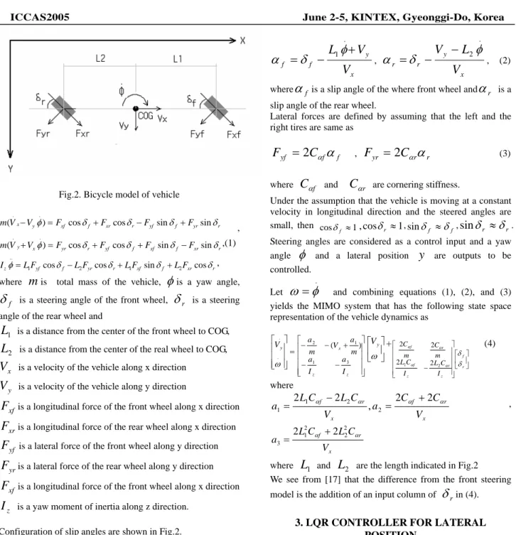
The vehicle is steered by both the front and the rear wheel. For simplicity, the vehicle dynamics is considered as a bicycle model as shown in Fig.2. The dynamic equations are derived based on the references [15,16].

Neural Network Control Technique for Automatic Four Wheel Steered Highway

Snowplow Robotic Vehicles

Seul Jung*, Ty Lasky**, and T. C. Hsia***

* Department of Mechatronics Engineering, Chungnam National University, Daejeon, Korea (Tel : +82-42-821-6876; E-mail: [email protected])

**Advanced Highway Maintenance and Construction Technology Center, University of California, Davis, USA (Tel : +1-530-000-; E-mail: [email protected])

***Department of Electrical & Computer Engineering, University of California, Davis, USA (Tel : +1-530-000-7440; E-mail: [email protected])

Abstract: In this paper, a neural network technique for automatic steering control of a four wheel drive autonomous highway

snowplow vehicle is presented. Controllers are designed by the LQR method based on the vehicle model. Then, neural network is used as an auxiliary controller to minimize lateral tracking error under the presence of load. Simulation studies of LQR control and neural network control are conducted for the vehicle model under a virtual snowplowing situation. Tracking performances are also compared for two and four wheeled steering vehicles.

ICCAS2005 June 2-5, KINTEX, Gyeonggi-Do, Korea

Fig.2. Bicycle model of vehicle

r yr f yf r xr f xf y x V F F F F V

m( φ) cosδ cosδ sinδ sinδ

. . + − + = − , r xr f xf f yf r yr x y V F F F F V

m( φ) cosδ cosδ sinδ sinδ

. . − + + = + ,(1) r xr f xf r yr f yf z LF LF LF LF

I φ 1 cosδ 2 cosδ 1 sinδ 2 cosδ

..

+ +

−

= ,

where

m

is total mass of the vehicle,

φ

is a yaw angle,

f

δ

is a steering angle of the front wheel,

δ

_r is a steering angle of the rear wheel and

1

L

is a distance from the center of the front wheel to COG,

2

L

is a distance from the center of the real wheel to COG,

x

V

is a velocity of the vehicle along x direction

y

V

is a velocity of the vehicle along y direction

xf

F

is a longitudinal force of the front wheel along x direction

xr

F

is a longitudinal force of the rear wheel along x direction

yf

F

is a lateral force of the front wheel along y direction

yr

F

is a lateral force of the rear wheel along y direction

xf

F

is a longitudinal force of the front wheel along x direction

z

I

is a yaw moment of inertia along z direction. Configuration of slip angles are shown in Fig.2.

Fig. 3 Slip angle model Slip angles are defined by

x y f f

V

V

L

+

−

=

. 1

φ

δ

α

, x y r r

V

L

V

. 2

φ

δ

α

=

−

−

, (2)

where

α

_f is a slip angle of the where front wheel and

α

_r is a slip angle of the rear wheel.

Lateral forces are defined by assuming that the left and the right tires are same as

f f yf

C

F

=

2

_α

α

,

F

_yr

=

2

C

_αr

α

_r (3) where

C

_αf and

C

_αr are cornering stiffness.

Under the assumption that the vehicle is moving at a constant velocity in longitudinal direction and the steered angles are small, then _{cos ≈1}

f δ ,cos

δ

_r ≈1, f f

δ

δ

≈ sin ,

sin

δ

_r

≈

δ

_r. Steering angles are considered as a control input and a yaw angle

φ

and a lateral position

y

are outputs to be controlled.

Let

.

φ

ω

=

and combining equations (1), (2), and (3)

yields the MIMO system that has the following state space representation of the vehicle dynamics as

= ⎥ ⎥ ⎥ ⎦ ⎤ ⎢ ⎢ ⎢ ⎣ ⎡ . . ω y V ⎥ ⎥ ⎥ ⎥ ⎦ ⎤ ⎢ ⎢ ⎢ ⎢ ⎣ ⎡ − − + − − z z x I a I a m a V m a 3 1 1 2 _{( )} ⎥ ⎦ ⎤ ⎢ ⎣ ⎡ ω y V ₊ ⎥ ⎦ ⎤ ⎢ ⎣ ⎡ ⎥ ⎥ ⎥ ⎥ ⎦ ⎤ ⎢ ⎢ ⎢ ⎢ ⎣ ⎡ − r f z r z f r f I C L I C L m C m C δ δ α α α α 2 1 2 2 2 2 (4) where x r f x r f

V

C

C

a

V

C

L

C

L

a

2

α

2

α

,

2

2

α

2

α 2 1 1

+

=

−

=

, x r f V C L C L a α α 2 2 2 1 3 2 2 + =

where

L

₁ and

L

₂ are the length indicated in Fig.2 We see from [17] that the difference from the front steering model is the addition of an input column of

δ

_rin (4).

3. LQR CONTROLLER FOR LATERAL

POSITION

The LQR control block diagram for lateral position tracking is shown in Fig. 4. The goal of the LQR control method is to minimize the following objective function

dt

Ru

u

Qx

x

J

T T

)

(

0

∫

∞

+

=

(5)

where

Q,

R

are the weighting matrices. Those

Q,

R

values are selected based on trial and error processes. The ultimate goal is to control the lateral position y.

Fig. 4. Lateral control block diagram The lateral position error is formed as

y

y

e

_y

=

_d

−

. (6) The yaw angle error is formed as

φ

φ

φ

=

d

−

e

. (7)

Those errors are multiplied by controller gains found by

the LQR control method. The controller inputs for the

front steering

u

_f

and the rear steering

u

_r

are defined

as

φ φ

e

k

e

k

u

y

=

yf y

+

r

,

φ φ

e

k

e

k

u

_r

=

_{yr y}

+

_r , (8)

where

k

_yf

,

k

_φf ,

k

_yr

,

k

_φr are controller gains obtained by the LQR algorithm. For simplicity, we have the relationship

u

=

δ

by not considering dynamics of a steering mechanism.

4. NEURAL NETWOK CONTROL

4.1 Neural network control structure

In this paper, we are implementing an on-line learning algorithm for the neural network. The idea is that a neural network compensates for uncertainties by minimizing the errors. The objective function is minimized in on-line fashion by adding compensating signals from the neural network to the LQR controller output. Control inputs are defined by adding neural network outputs

u

_N to (8) as

Nf y f

=

u

+

u

δ

, Nr r

=

u

φ

+

u

δ

, (9)

where

u

_Nf

,

u

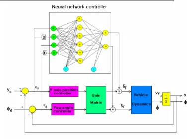
_Nr are neural network outputs.

Fig. 5 shows the neural network control block diagram. Neural network outputs are added to the LQR controller outputs. At each sampling time, weights of the neural network are updated to generate new compensating signals. The key issue here is how to implement on-line learning and control. To achieve on-line control, certain fast computing power will be required.

Fig.5. Neural network control block diagram

4.2 Neural network learning

For neural network learning, we have used a general feed-forward structure that has an input layer, a hidden layer, and an output layer shown in Fig. 6. For the control application, 4 input buffers, 6 hidden units and 2 output units are used. Increasing the number of inputs and hidden units did not help to improve the performance in our simulations.

Fig. 6. Neural network structure

For a nonlinear function at a hidden layer and an output layer we have used the hyperbolic tangent function as

) exp( 1 ) exp( 1 ) ( x x x f − + − − = . (10)

Here, neural network learning algorithm is derived. Since we are doing on-line learning and control, selecting the training signal is very important. Typically, the bicycle model of the vehicle is a squared MIMO system that two control inputs has to satisfy two different outputs simultaneously.

If

(

,

,

,

,

,

,

)

.. . .. .

δ

φ

φ

φ

y

y

y

f

is the system dynamics,

ICCAS2005 June 2-5, KINTEX, Gyeonggi-Do, Korea

N r y yf f y yf

u

y

y

y

f

e

k

e

k

e

k

e

k

−

=

+

+

+

)

,

,

,

,

,

,

(

.. . .. .

δ

φ

φ

φ

φ φ φ φ , (11) where

u

=

[

u

_Nf

u

_Nr

]

Tand

δ

=

[

δ

_f

δ

_r

]

T.

So here we define the training signal of neural network as the sum of outputs of PD controllers.

φ φ φ φ

e

k

e

k

e

k

e

k

v

=

_{yf y}

+

_f

+

_{yr y}

+

_r . (12)

The objective function is defined as

2

2 1 v

E= (13)

Differentiating (13) with respect to weights, we have

w

u

v

w

v

v

w

v

v

E

w

E

N

∂

∂

−

=

∂

∂

=

∂

∂

∂

∂

=

∂

∂

. (14)

The update equation in the back propagation algorithm is

)

1

(

)

(

+

Δ

−

∂

∂

=

Δ

v

w

t

w

u

t

w

η

N , (15) ) ( ) ( ) 1 (t wt wt w + = +Δ

. (16)

5. SIMULATION STUDIES

5.1 Vehicle model

The following parameters of the vehicle are used for simulation studies.

Table 1. Parameters of the vehicle

M(kg) Iz(Kgmsec^2) Cf, Cr(Kg/rad) L1(m) L2(m)

2612.7 810.2 4082.4 1.45 1.94

Here we assume the constant longitudinal velocity at

V

_x= 10.973km/sec.

Then the state space representation of (4) becomes

= ⎥ ⎥ ⎦ ⎤ ⎢ ⎢ ⎣ ⎡ . . ω y V ⎥ ⎦ ⎤ ⎢ ⎣ ⎡ − − − 3453 . 19 4884 . 0 5030 . 9 625 . 0 ⎥ ⎦ ⎤ ⎢ ⎣ ⎡ ω y V + ⎥ ⎦ ⎤ ⎢ ⎣ ⎡ ⎥ ⎦ ⎤ ⎢ ⎣ ⎡ − r f δ δ 5051 . 19 6212 . 14 125 . 3 125 . 3

Controller gains are selected by the LQR method for the simulation studies. We have found the controller gains as

⎥ ⎦ ⎤ ⎢ ⎣ ⎡ − − = 0492 . 0 0849 . 0 0194 . 0 0238 . 0 K .

The vehicle is required to follow the desired lateral trajectory. A load is assumed to be present. The desired lateral position is 3m.

5.2 LQR control method

Fig. 7 shows the tracking performance of LQR controllers. Different tracking responses of selecting gains as ⎥ ⎦ ⎤ ⎢ ⎣ ⎡ = 1 0 0 1 Q and _⎥ ⎦ ⎤ ⎢ ⎣ ⎡ = r r R 0

0 _{are plotted. We see that the}

large value r gives the good tracking performance in the aspect of overshoot and settling time before 15 seconds. But when load is present after 15 seconds, tracking performance became the worst. We also altered the value of Q matrix, but Q=I is found to be the best. We found that the value of Q matrix is more sensitive than that of R. Small change in Q results in bad tracking performance. Since this is a coupled system, gain changes affect both tracking performances of the position and the yaw angle. It is clearly shown that offset tracking errors occur when load appears as shown in Fig. 7.

Fig. 7. Lateral position tracking by LQR controllers Next is the comparison result of lateral control between two wheel drive and four wheel drive vehicles. We see here from Fig 8. that both cases show tracking errors when load is present. However, a less lateral position tracking error has been observed for a four wheel drive steering vehicle even though a two wheel drive vehicle shows no overshoot at a transient response. This explains that the four wheel drive vehicle system pushes more to the lateral direction to achieve the fast settling time when load is present. We also observed that a two wheel drive vehicle become unable to track desired trajectory with other LQR controller gains.

0 5 10 15 20 25 30 35 40 45 50 1.8 2 2.2 2.4 2.6 2.8 3 3.2 3.4 3.6 time (sec) Y pos it ion ( ft )

Fig.8. Lateral position tracking of two(dash line) and four(solid line) wheel drive vehicles

1. Snowplowing load is 138N.

To minimize those tracking errors, the same experiment has been conducted by adding a neural network controller. For the neural network parameters,

9

.

0

,

000055

.

0

=

=

α

η

are used and those values are

optimized by trial and errors. Fig. 9 shows the lateral position tracking results for the LQR control method and the neural network control method. We clearly see by comparison that a tracking error is minimized by the neural network controller. Fixed LQR controller cannot minimize the tracking error when load is present after 15 seconds.

0 5 10 15 20 25 30 35 40 45 50 2 2.2 2.4 2.6 2.8 3 3.2 3.4 3.6 time (sec) Y po s it ion (f t)

Fig. 9. Lateral position tracking of LQR(dotted line) and Neural network control(solid line).

2. Snowplowing load is 691N.

Now the load has been increased after 15 seconds. We see from Fig. 10 that the neural network controller outperforms in tracking performance while the LQR controller cannot recover from deviation. Even though load is increased 5 times, a position tracking error is compensated fast by the neural network controller.

0 5 10 15 20 25 30 35 40 45 50 2 2.2 2.4 2.6 2.8 3 3.2 3.4 3.6 time (sec) Y pos it ion ( ft ) NN Control LQR Control

Fig. 10. Lateral position tracking.

6. CONCLUSIONS

This paper presented lateral tracking control simulation studies of the autonomous four wheel drive vehicle. The simplified bicycle model has been used for simulation studies.

addition, neural network controllers are introduced to minimize tracking errors due to the present load.

Simulation studies show that the neural network controller outperforms over the LQR controller under present load conditions. We observed that the two wheeled drive vehicle often went unstable when load is present. The four wheeled drive vehicle performs better than two wheel drive vehicle specially when load is present. It turns out that the neural network controller is robust to variation of load.

ACKNOWLEDGMENTS

The author Seul Jung has been a sabbatical leave at

University of California, Davis for 6 months from

March to August of 2004. Dr. Seul Jung would like to

thank both Chungnam National University and the

University of California, Davis for their sincere help.

REFERENCES

[1] T. A. Lasky and B. Ravani, “Sensor based path Planning and Motion Control for a Robotic System for Roadway Crack Tracking”, pp. 609-622, IEEE Trans. On Control Systems Technology, col. 8, No. 4, 2000

[2] Hyun Taek Cho, Poong woo Jeon, and Seul Jung,

“Implementation and control of a roadway crack tracking mobile robot with force regulation”, IEEE Conf. On Robotics and Automations, pp. 2444-2449, 2004 [3] R. T. O’Brien, P. A. Iglesias, and T. J. Urban, “Vehicle

lateral control for automated highway systems”, IEEE Trans. On Control Systems Technology, pp. 266-273, 1996

[4] S. Y. Yang, S. T. Park, J. H. Jeong, B. R. Park, “Development of intelligent automated driving control system (lateral control)”, KORUS’99, pp. 334-337, 1999

[5] S. J. Hong, J. Y. Choi, Y. I. Jeong, K. Y. Jeong, M. H. Lee, K. T. Park, K. S. Yoon, and N. S. Hur, “Lateral control of autonomous vehicle by yaw rate feedback”, IEEE Symposium on Industrial Electronics, pp. 1472-1476, 2001

[6] R. H. Byrne, C. T. Abdallah, and P. Dorato,

“Experimental results in robust lateral control of highway vehicles”, IEEE Control Systems Magazine, pp. 70-76, 1997

[7] Longitudinal and lateral control of heavy duty trucks for automated vehicle following in mixed traffic: Experimental results from the CHAUFFEUR project”, IEEE Conf. On Control Applications, pp. 1348-1352, 1999

[8] O. Pages, A. E. Hajjaji, R. Ordonez, “H Tracking _∞ for Fuzzy Systems with an Application to Four Steering of Vehicles”, IEEE Conf. On , pp. 4364-4369, 2003 [9] A. B. Will, M. C. Teixeira, and S. H. Zak, “Four Wheel

Steering Control System Design Using Fuzzy Models”, IEEE Conf. On Control Applications, pp. 73-78, 1997 [10] L. Cai, A. B. Rad, and K. Y. Cai, “A robust fuzzy PD

controller for automatic steering control of autonomous vehicles”, IEEE Conf. On Fuzzy Systems, pp. 549-554, 2003

[11] S. Jung and T. C. Hsia, “Neural Network Inverse

Control Techniques for PD Controlled Robot

Manipulator”, ROBOTICA, pp. 305-314, vol. 19, No 3, 2000

ICCAS2005 June 2-5, KINTEX, Gyeonggi-Do, Korea

“Feedback error learning neural network for trajectory control for of a robotic manipulator”, Neural Networks, vol. 1, pp. 251-265, 1988

[13] Sungsu Kim and Seul Jung, Hardware Implementation of a real time neural network controller with a DSP and an FPGA, IEEE Conf. On Robotics and Automations, pp. 4639-4644, 2003

[14] S. Jung and S. B. Yim “Experimental studies of neural network control technique for nonlinear systems”, ICASE, pp. 918-926, vol. 7, no. 11, 2001

[15] H. T. Cho and S. Jung, “Balancing and Position control of an Inverted pendulum on an X-Y Plane using Decentralized neural networks”, Proceedings of the 2003 International Conference on Advanced Intelligent Mechatronics, pp. 181- 186, 2003.

[16] H. T. Cho and S. Jung, “Neural network position tracking control of an inverted pendulum by an x-y table robot”, International Conference on Intelligent Robots and Systems, pp. 1210-1215, 2003

[17] J. Y. Wong, “Theory of Ground Vehicles”, John Wiley & Sons, 1978

[18] S. H. Yu and J. J. Moskwa, “A Global Approach to Vehicle Control: Coordination of Four Wheel Steering and Wheel Torques, Journal of Dynamic Systems, Measurement, and Control, Vol. 116, pp. 659-667, 1994