Collision-free Path Planning Using Genetic Algorithm

유전자 알고리즘을 이용한 충돌회피 경로계획

Collision-free Path Planning Using Genetic Algorithm

이동환^*, 조연^**, 이홍규^**

Dong-Hwan Lee^*, Zhao Ran^** and Hong-Kyu Lee^**

요 약

본 논문은 로봇 충돌회피 경로계획의 문제점을 해결하기 위해 진화된 모델에 근거한 새로운 경로탐색 전략 을 소개한다. 최적화된 지능형 검색 방법으로 잘 알려진 유전자 알고리즘을 이용하여 로봇 경로계획 방법을 설 계하였다. 염색체 안에 있는 유전자 인자로 경로점을 고찰해보면 주어진 맵에 대한 가능한 해법이제공된다. 생 성된 염색체 간의 거리가 먼 경우 유사한 염색체에 대한 적합도로 간주할 수 있다. 경로계획에 있어 본 논문에 서 제안한 유전자 알고리즘의 유효성을 증명하기위해 다양한 방법으로 시뮬레이션을 실시하였으며, 제안한 경 로 검색 방법은 정지된 장애물이나 복잡한 장애물에도 사용될 수 있음을 증명하였다.

Abstract

This paper presents a new search strategy based on models of evolution in order to solve the problem of collision-free robotic path planning. We designed the robot path planning method with genetic algorithm which has become a well-known technique for optimization, intelligent search. Considering the path points as genes in a chromosome will provide a number of possible solutions on a given map. In this case, path distances that each chromosome creates can be regarded as a fitness measure for the corresponding chromosome. The effectiveness of the proposed genetic algorithm in the path planning was demonstrated by simulation. The proposed search strategy is able to use multiple and static obstacles.

Key words : mobile robot, path planning, genetic algorithm

* 한국폴리텍IV대학

** 한국기술교육대학교(Dept. of Electrical and Electronics Engineering, Korea University of Technology and Education) ‧ 제1저자 (First Author) : 이동환

‧ 투고일자 : 2009년 9월 25일

‧ 심사(수정)일자 : 2009년 9월 28일 (수정일자 : 2009년 10월 23일) ‧ 게재일자 : 2009년 10월 30일

I. Introduction

In the past two decades, different conventional methods have been developed to solve the path planning problem, such as the cell decomposition, road map and potential field [1]. Most of these methods

were based on the concept of space configuration [2-3]. These techniques show lack of adaptation and a non robust behavior. To overcome the weakness of these approaches researchers explored variety of solutions [4]. There are three major concerns in regard to robot path planning problems; efficiency, safety and

accuracy. The efficiency of the algorithm is considered as an important matter since one of the main concerns is to find the destination in a short time. Accordingly, a desirable path should result from not letting the robot waste time taking unnecessary steps or becoming stuck in local minimum positions [5]. Furthermore, a desirable path should avoid all known obstacles in the area. This safety issue is another critical part of the algorithm. Once the optimum collision-free path is constructed, then it is a matter for the robot to accurately follow the pre-determined path. The main scope of the path planning problem involves the efficiency and safety issues [6].

Researches with various methods used to solve the path planning problem may be divided into two categories. One is the environment type which has static and dynamic, another is the kinds of the path planning algorithms (i.e., global or local). The global path planning algorithms requires a complete knowledge about the search environment and that all terrain should be static. On the other hand, local path planning means that path planning is being implemented while the robot is moving; in other words, the algorithm is capable of producing a new path in response to environmental changes [7].

Genetic algorithms (GA) are stochastic search methods and usually consist of a finite repetition of three steps at each generation: selection of the parent chromosomes, recombination using crossover and mutation operations, and a fitness function that describes the goodness of individual members of each generation [8], [9]. Considering via points as genes in a chromosome will provide a number of possible solutions on a grid map of paths. In this case, path distances that each chromosome creates can be regarded as a fitness measure for the corresponding chromosome.

Our main goal in this paper is to demonstrate the effectiveness of the proposed GA in the problem that control the robot moving in an environment which has

number of static obstacles with various sizes. The rest of this paper is organized as follows: Section II gives a background and related works. Section III describes the problem of the path planning for mobile robot in our paper. Section IV describes the algorithm design and fitness function and the results of the proposed algorithm. Conclusions are presented in Section V.

Ⅱ. Related Work

Genetic algorithms (GAs) are biologically inspired search methods which are loosely based on molecular genetics and natural selection. The synthesis of the ideas of Charles Darwin on evolution and natural selection, Mundelein genetics and molecular biology is often called neo-Darwinism. Darwin pointed out in The Origin of Species [10] that the natural consequence of the rule that like produces like (and that like is not identical) combined with the tendency of some progeny themselves to reproduce more successfully, is that a population over a period of time may change. In doing so then it would, on average, change such that members of future generations in the milieu of prior generations would naturally have a higher reproductive success rate. He did not define the mechanisms by which the change is coded. The importance of selection and the role of the gene in evolution are stressed by Dawkins in two popular and influential books, The Selfish Gene and The Blind Watchmaker [11, 12].

Path planning is an important issue in mobile robotics. In an environment with obstacles, path planning is to find a shortest collision-free path for a mobile robot to move from a start location to a target location. However, this problem includes several difficult phases that need to be overcome, such as obstacle avoidance, position identification, and so on.

Many different methods achieving varying degrees of success in a variety of conditions or criteria of

motion and environments have been developed.

Researchers distinguish between various methods used to solve the path planning problem according to two factors, 1) the environment type (i.e., static or dynamic, 2) the path planning algorithms (i.e., global or local). The static environment is defined as the environment which doesn’t contain any moving objects; while the dynamic is the environment which has dynamic moving objects (i. e., human beings, moving machines and moving robots). The global path planning algorithms requires a complete knowledge about the search environment and that all terrain should be static. On the other hand, local path planning means that path planning is being implemented while the robot is moving; in other words, the algorithm is capable of producing a new path in response to environmental changes

Ⅲ. Problem Description

The path planning problem discussed in this paper is that the robot can move from the start location to the target location with a static environment. The mobile robot moves in a closed workspace. This area is described by 2-D map (30×30 square maps in this paper) and the size of map can be changed. The map includes a finite number of static obstacles and a set of via points to help the robot in avoiding obstacles.

The obstacles are considered a circle and the radius can be changed arbitrarily while the robot was considered as a point. The position and amount of the obstacles can be selected arbitrarily in the map. The purpose of the proposed algorithm is to find a suitable collision-free path with shortest length for a robot to move from a start location to a target location.

The path planning problem has two major parts, that is, obstacle avoidance and shortest path length.

New chromosomes were generated in every generation.

Even if the performance based on path distance of a

new chromosome is acceptable, it could be a useless solution if the corresponding path passes through any of the obstacles. In order to make sure that via points cannot lie on any obstacle, the distance between the center of the obstacle and any via point must longer than the radius of obstacle. Similarly, if the distance between the center of the obstacle and the proposed segments is longer than the radius of obstacle one can make sure that the path will not pass through the obstacles.

A chromosome corresponds to possible solution of the optimization problem. Thus each chromosome represents a path which consists of straight line segments as the sequence of points with the first node indicating the starting location of the first segment, followed by via points between segments, and the last point indicating the ending point of the last segment, which is the target location.

Ⅳ. Proposed Path Planning Algorithm

A chromosome corresponds to possible solution of the optimization problem. Thus each chromosome represents a path which consists of straight line segments as the sequence of points with the first node indicating the starting location of the first segment, followed by via points between segments, and the last point indicating the ending point of the last segment, which is the target location.

4-1 Coding Format

We assume that the robot can move to any location in the map which means that the abscissas and ordinates can be located randomly at any point in the 30×30 square maps. And there is n-2 via points to from the start location to the target location. All the coordinates are real-valued number and the coordinate of the start point, (x_{i, 0},y _{i, 0}) and the coordinate

of the target point, (x_{i,n- 1},y_{i,n- 1}).

,0 ,0 ,1 ,1 , 1 , 1

(( , ), ( , ),...( , ))

i i i i i i n i n

R = x y x y x _- y _- (1)

We can the corresponding chromosome as the

^{ni =(xi,0,xi,1,...,xi n,-1,yi,0,yi,1,...,yi n,-1)} (2) 4-2 Fitness Function

The fitness function is the base of the algorithm and it can impact the speed of convergence directly. A good fitness function can save much time and obtain a satisfactory result. In our proposed fitness function has 3 key parts;

‐ The summation of the length of all the path segments, L(ν _i)

‐ The summation of the distance between the radius of every obstacles and every via points, D(ν_i)

‐ and the distance between the center of obstacles and the path, S(ν _i)

The fitness function,

) ( ) ( )

( ) 1 (

3 2

1 i i i

i L v D v S v

v

F =w +w +w

　(3)

where ω₁,ω ₂ and ω ₃ are weight coefficients.

1) L(ν _i) : it is calculated by summing the length of all the path segments one by one.

å

-

=

+

+ + -

-

=

2

0

2 1 , , 2 1 ,

, ) ( )

( )

(

n

j

j i j i j

i j i

i x x y y

v

L (4)

2) D(ν _i) : the summation of the distance between the radius of possible obstacles and every via points in the map. We designed the penalty function

is as following

å å

= -

=

=

m

k k j n

j

i d

v D

1 , 1

0

)

( 　　　　 　(5)

A penalty function was required to insure that via points should not be lying on the obstacle. Assume that the amount of obstacles and the location can be get from the sensors on the Robot. A feasible path must insure that any part of the robot should not collide with the obstacles, that is, the distance between the robot and the edge of the obstacle must longer than the minimum safe distance. That is, the distance between the center of the obstacle and via points must longer than the radius of the obstacle. Note that, the coordinate of the center of obstacle is (xo _k,yo _k) where k is the number of the obstacles and

k= 1,2,⋯,m^.

When via points lying on the obstacles,

d _j,k= (x_i,j-xo _k) ²+(y_i,j-yo _k) ² (6) Others, d _j,k= 0.

3) S(ν _i) : it is required to insure that the path should not intersect with the coverage of obstacles.

The distance between the center of obstacles and the segments of the path must longer than the radius of obstacles.

Fig 1. Distance between the center of obstacles and the path

In Fig 1. P _{j- 1}^, P_j ^and P _{j+ 1} are three via points of the path ν _i, and the corresponding coordinates are (x_{i,j- 1},y _{i,j- 1}), (x_i,j,y _i,j) and (x_{i,j+ 1},y_{i,j+ 1}). Two circles O _k ^and O _{k- 1} are obstacles where the coordinates of the center respectively are (xo _k,yo _k) and (xo _{k- 1},yo _{k- 1}). l _k,j

and l _{k,j+ 1} are respectively the distance between the obstacle O _k and the segment P _{j- 1}P_j ^and the segment P_jP_{j+ 1}. Thus, the proposed distance,

l _k,j, can be calculated as

_{ } 

^   _{ }^ _{  } _{ }^

 _{ } _{  }_ _{  } _{ }_ _{ }_{  } _{  }_{ }

(7) We defined,

{^ll^''k_k^,_,^j_j^{= 0 ,}= 1 ,wher e l^{wher e l}_k^k_,^,_j^j≤^>RR^o_o Where R ₀ is the radius of the obstacles.

å å

= -

=

=

m

k j k n

j

i l

v S

1 ' , 1

1

)

( (8)

In addition, when the segment created between P _{j- 1} ^and P_j did not pass through the obstacle,

the segment was located outside of obstacles. In this case, we do not need to consider the distance between the center of the obstacle and the proposed segment, that is l^'_k,j= 0.

The fitness of each chromosome can be calculated in terms by F(ν _i). The bigger that the value of F(ν _i) is the better that corresponding chromosome will be. Thus this fitness function can easily be extended to penalize paths for traversing certain terrain or modified to push paths away from obstacles. As mentioned previously, a genetic algorithm method can easily change the search criteria without modifying the entire planning algorithm.

4-3 GA Operators

The program sequence of the proposed algorithm is given by:

Initialize the parameters of environment Initialize the parameters of genetic algorithm Do for generation = 1, 2, … N (N; MAXGEN) Evaluate the fitness for each chromosome in current population using the fitness function

Rank the population using the fitness values Apply selection process between the current chromosomes

Apply crossover process with the given probability Apply the mutation process with the given probability

Generate the new population Gen = Gen + 1

End for

Output the best individual

The first step in a genetic algorithm is to create an initial population consisting of random individuals. In this paper, the function ‘crtrp’ was used to creating the initial population.

1) Selection

After represent the chromosomes, the second decision to make in using a genetic algorithm is how

to perform selection. We used stochastic universal sampling (SUS) in our algorithm, SUS is a single-phase sampling algorithm and spins the wheel once—but with N equally spaced pointers, which are used to select the N parents. At each generation all the chromosomes will be updated by their fitness. In other words, if a particular chromosome has better fitness (bigger value of ) than other chromosomes, then that particular chromosome is more likely to win the competition and clone itself. Thus, by using the selection function ‘sus’, a chromosome with good fitness has a much higher probability than other inferior chromosomes to appear in the next generation.

2) Crossover

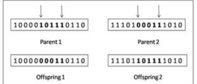
It could be said that the main distinguishing feature of a GA is the use of crossover. For multi-point crossover, m crossover positions, where the crossover points and is the length of the chromosome, are chosen at random with no duplicates and sorted into ascending order. Then, the bits between successive crossover points are exchanged between the two parents to produce two new offspring. In this paper, we used double-point crossover operator,

‘xovdp’ which is a specific case of multi-point crossover with the number of crossover positions is 2 with the form NewChrom = xovdp (OldChrom,P _c^).

Where ‘OldChrom’ are the parent chromosomes and P_c is the probability of crossover. This operator performs double-point crossover between pairs of individuals contained in the current population,

‘OldChrom’, according to the crossover probability, P_c, and returns a new population after mating,

‘NewChrom’. Each row of ‘OldChrom’ and

‘NewChrom’ corresponds to one individual. By using this operator, both parent paths was divided randomly into three parts respectively and recombined. As shown in Figure 2, the middle part of the first path between crossover bit positions and the middle part of the second path are exchanged to produce the new

children. The crossover bit positions are selected randomly along the chromosome in each generation.

Fig 2. Example of double-point crossover

3) Mutation

In GA mutation is usually considered as a background operator, the role of mutation is often seen as providing a guarantee that the probability of searching any given string will never be zero and acting as a safety net to recover good genetic material that may be lost through the action of selection and crossover. The goal of the mutation operators is to increase population diversity of the chromosomes. We used ‘mutbga’ which takes the real-valued population, OldChrom, mutates each variable with given probability and returns the population after mutation, NewChrom = mutbga(OldChrom, FieldDR,P _m⁾ takes the current population, stored in the matrix OldChrom and mutates each variable with probability by addition of small random values. Where ‘FieldDR’

is a matrix containing the boundaries of each variable of an individual, P _m is the probability of mutation.

Ⅴ. Simulation and Conclusion

5-1 Simulation Results

In order to demonstrate the effectiveness of genetic algorithm, different conditions with different number and radius of obstacles have been set up to create variety of experiments. In every figure, the circles represent the obstacles, and the “+” objects represent

via points. All the experiments were done with MATLAB 7.0 and GA toolbox. In this section, varies of experiments with different environment were performed. Such as different number of the obstacles, radius of obstacles (Ro) and different number of via points. Different GA parameters were also used, that is, different probability of crossover and mutation, and different maximum number of generation (MAXGEN).

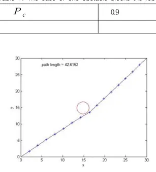
Table 1. The case of one obstacle blocks the robot

P_c 0.9

Fig 3. Result with one obstacle when Ro = 2

Table 2. The case of two obstacles in the map

P_c 0.9

Fig 4. Result with two obstacles when Ro = 2, MAXGEN = 4000

Table 3. The case of multiple obstacles used in the map

P _c 0.9

P _m 0.01

Number of obstacles 8

R ₀ 2

Number of via points 15

Path Length 44.75

MAXGEN 4000

Fig 5. Result with multiple obstacles when MAXGEN

= 3000

At every generation, the algorithm needs calculate the fitness value of every individual and select the better ones with high fitness value for evolving.

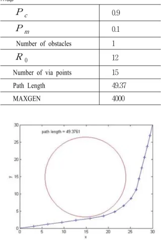
Theoretically, when there is a large obstacle locates in the map, as the number of via points increased, the path is much smoother and closer to the edge of the obstacle. Furthermore, apparently when there are a few number of obstacles lie in the map, the algorithm can find an optimum path easily.

Table 4. The case of a large obstacles used in the map

P_c 0.9

P_m 0.1

Number of obstacles 1

R ₀ 12

Number of via points 15

Path Length 49.37

MAXGEN 4000

Fig 6. Result with a large obstacle when Ro = 12, MAXGEN = 4000

Contrarily, when there are multiple obstacles the potential paths will be very complex. In this case, if the number of via points is very small, it hardly to get a collision-free path. So, more obstacles require more via points. As the number of via points increased, the length of the chromosome increased too. According to these experiments we can see that when R _o was not large the influence of R _o to the algorithm was not obvious.

When R _o

was very large, was increased to 8 and 12, P_m increased to 0.05 and 0.1 respectively.

Mutation operation can improve the diversity of individuals. In the path planning problem, as P _m increased, via points have a higher probability to mutate to the free space of the map to avoid collision

with the obstacles. In these two experiments, because of the higher probability of mutation, the variety of potential paths increased, so large number of maximum generation or computation time required.

The relationship between the parameters was shown as follow.

That is,

■　Larger number of obstacles require larger number of generations and longer computation time, and may require more via points sometimes.

■　More via points lead to shorter path length but longer computation time.

■　 Larger number of generations (less than MAXGEN) or computation time may lead to better solutions.

■　 Larger radius of obstacle requires large probability of mutation and longer computation time

Fig 7. Result with relationship between parameters of experiment

5-2 Conclusion and Future work

In this paper we presented a path planning program in static environment based on Genetic Algorithm and global path planning method. In order to demonstrate the effect of genetic algorithm, different conditions of environment and different GA parameters have been set up to create variety of experiments. With the use

of the initialization of chromosomes, fitness function, GA operators and parameters for the Genetic Algorithm, it is possible to generate feasible paths in the experimented results in the simulation. The simulation performed using the coding format in two dimensions. It has been demonstrated that proposed methods can get satisfactory results for the path planning problem, It was shown that the choice of parameters for the experiment effected the time to execute the compute and the quality of the solution (length of the path).

In this paper, the enactment of the obstacles was static. So applying this algorithm in an environment with dynamic obstacles can be a challenging topic for future work, e.g. football robot. In addition, more research for the path planning problem can be done by applying this algorithm to a real robot.

Reference

[1] B. Graf, J. M. Hostalet Wandosell, “Flexible path planning for non-holonomic mobile robots”, In Proc. 4th European workshop on advanced Mobile Robots (EUROBOT’01)., Fraunhofer Inst.

Manufact. Eng. Automat (IPS). Lund, Sweden,pp.

199-206, Sept. 19-21, 2001.

[2] J. C. Latombe, “Robot Motion Planning”. 1sted, Boston, UK, MA: Kluwer Academic Publishers (Published by Springer), 1991.

[3] Kyung Min Han, "Collision Free Path Planning Algorithms For Robot Navigation Problem", Master Thesis, the Faculty of the Graduate School, University of Missouri-Columbia, 2007.

[4] A. Elshamli, H. A. Abdullah and S. Areibi,

“Genetic algorithm for dynamic path planning”.

IEEE Vol.2, May 2-5, pp: 677-680, 2004.

[5] S. Lee and G. Kararas, “Collision-Free Path Planning with Neural Networks”, 1997 IEEE International Conference on Robotics and

Automation.

[6] D. Huh, J, Park, U. Huh, H. Kim, “Path Planning and Navigation for Autonomous Mobile Robot”, IECON 02 IEEE annual conference.

[7] K. H. Sedighi, K. Ashenayi, T. W. Manikas, R.

L. Wainwright, and H. M. Tai, “Autonomous Local Path Planning for a Mobile Robot Using a Genetic Algorithm,” in Congr. Evol. Comput, Vol. 2, pp. 1338-1345, CEC2004.

[8] Hong K.. Lee, and Gordon K. Lee, “Convergence Properties of Genetic Algorithms”, Proc. of the ISCA, pp. 172-176, Mar. 2004.

[9] Damion Gastelum, and Hong K. Lee, and Gordon K. Lee, et al, “The Development of a Testbed for Evolutionary Learning Algorithms For Mobile Robotic Colonies”, 2004 International Symposium on Collaborative Technologies and Systems, pp.

212-217, Jan. 2004.

[10] C. Darwin, “On the origin of species by means of natural selection, or the preservation of favoured races in the struggle for life,” Second ed. London:

John Murray, 1859.

[11] R. Dawkins, “The Selfish Gene”. Oxford: Oxford University Press, 1976.

[12] R. Dawkins, “The Blind Watchmaker”. Oxford:

Longman, 1986. [11] D.F. Ferraiolo and D.R.

Kuhn, "Role Based Access Control," In Proc. of the 15th National Computer Security Conference, Oct, 1992 “The small screen [TV to Mobile Devices],” IEE Rev., vol. 49, no. 10, pp. 38-41, Oct. 2003.

이 동 환 (李東奐)

1999년 2월 : 한국기술교육대학교 전기공학과(공학사)

2006년 2월 : 한국기술교육대학교 전기공학과(공학석사)

2007년 3월~현재 : 한국기술교육 대학교 전기공학과 박사과정 2006년 2월~현재 폴리텍대학 교수 관심분야 : 유전자알고리즘, 로보틱스,

조 연 (Ran Zhao)

2006년 7월 : Shandong University (Bachelor of Information and

Computation Science/공학사) 2009년 8월 : 한국기술교육대학교 (Master of Electrical Engineering/

공학석사)

관심분야 :유전자 알고리즘, 선형시스템,

이 홍 규 (李弘珪)

1977년 2월 서울대학교 전자공학과 공학사

1979년 8월 서울대학교 전자공학과 공학석사

1989년 8월 서울대학교 전자공학과 공학박사

1979년 3월 - 1992년 2월 국방과학 연구소 선임연구원

1994년 3월~1995년 2월 독일 뮌헨공대 방문교수 2003년 1월~2004년 1월 샌디에고 주립대 방문교수 1992년 3월~현재 한국기술교육대학교 교수

관심분야 : 진화로봇, 유전자알고리즘, 로보틱스, 전자전