Sensitivity analysis of satellite-retrieved SST using IR data from COMS/MI

1. Introduction

Sea Surface Temperature (SST) is the sea temperature close to the ocean’s surface and affects the Earth’s atmosphere as an important parameter for monitoring the climate circulation and change (Park et al., 2013).

The global determination of climate change through the SST is an important aim of satellite remote sensing (Park et al., 2013; Smith et al., 1996). In previous study, the SST estimation from satellite have been performed for the accuracy improvement. To evaluate the quality of SST production, Park et al., (2011) assessed the SST error from between the National Oceanic and

Atmospheric Administration (NOAA) satellite (NOAA-15, 17, 18 and 19) and the drifting data.

O’Carroll et al (2012) produced the SST from the Meteorological Operation (MetOp)/Infrared Atmospheric Sounding Interferometer (IASI) and Advanced Very High Resolution Radiometer (AVHRR) sensors.

Although the SST measurement need accurate data for climate model, the SST from satellite still has biases from the error in specifying retrieval coefficients from either forward modeling or instrumental biases (Merchant and Borgne, 2004; Merchant et al., 2009).

Furthermore, to produce high quality of the SST products, radiometric calibration was also conducted

Sensitivity analysis of satellite-retrieved SST using IR data from COMS/MI

Eun-bin Park, Kyung-soo Han

Jae-hyun Ryu and Chang-suk Lee Department of Spatial Information Engineering, Pukyong National University

Abstract : Sea Surface Temperature (SST) is the temperature close to the ocean’s surface and affects the Earth’s atmosphere as an important parameter for the climate circulation and change. The SST from satellite still has biases from the error in specifying retrieval coefficients from either forward modeling or instrumental biases. So in this paper, we performed sensitivity analysis using input parameter of the SST to notice that the SST is most affected among the input parameter. We used Infrared (IR) data from the Communication, Ocean, and Meteorological Satellite (COMS)/Meteorological Imager (MI) from April 2011 to March 2012. We also used the Global Space-based Inter-Calibration System (GSICS) correction to quality of the IR data from COMS.

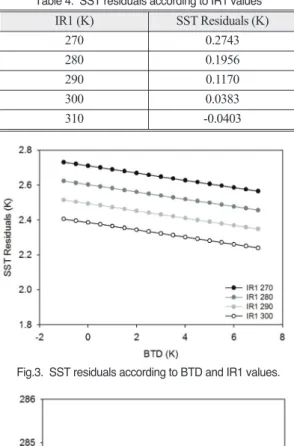
SST was calculated by substituting the input parameters; IR data with or without the GSICS correction. The results of this sensitivity analysis, the SST was sensitive from -0.0403 to 0.2743 K when the IR data were changed by the GSICS corrections.

Key Words : SST, COMS/MI, sensitivity analysis, GSICS correction http://dx.doi.org/10.7780/kjrs.2013.29.6.1

Received October 17, 2013; Revised November 5, 2013; Accepted November 7, 2013.

†

Corresponding Author: Kyung-soo Han ([email protected])

This is an Open-Access article distributed under the terms of the Creative Commons Attribution Non-Commercial License (http://creativecommons. org/licenses/by-nc/3.0) which permits unrestricted non-commercial use, distribution, and reproduction in any medium, provided the original work is properly cited

ISSN 2287-9307 (Online)

by Sohn et al. (2010). To assess the quality of products or input data, sensitivity analysis of input parameters from atmospheric correction was performed by Lee and Han (2009) by using fixed values of parameters except one parameter: object of analysis. Ha et al. (2006) were also conducted the sensitivity analysis about input parameter of aerosol, especially IR channel. Changes of Brightness Temperature Difference (BTD) were analyzed by changing the seven variables. In this paper, to assess the sensitivity of the SST products, we performed sensitivity analysis using input parameter of the SST. We used the Infrared (IR) data from the Communication, Ocean, and Meteorological Satellite (COMS)/Meteorological Imager (MI) from April 2011 to March 2012. And the quality of level 1 data, we used the Global Space-based Inter-Calibration System (GSICS) correction, which initiated by the World Meteorological Organization (WMO) in 2005 (Goldberg et al., 2011). We produced the SST by substituting the input parameters; IR data with or without the GSISC correction and viewing zenith angle (VZA) and monitored changes of values of the SST. Finally, we assessed that how sensitive is the SST, which were calculated by changing the input parameters; such as by changing at 10 K intervals of the IR1 data.

2. Data and Method

Sensitivity analysis of SST in this paper included the GSICS correction, which provides coefficients to the user to applying their geostationary satellite (Goldberg et al., 2011). IR data from COMS/MI were corrected by the GSICS correction for quality of input parameter and effects on SST. The location of the GSICS correction for IR channels from COMS/MI and IASI were at the latitude of 40°S ~ 40°N, the longitude of 63

~ 192°E. Match-up data set were composed up the COMS/MI and IASI data, whose locations were same each other. The equation for the GSICS correction of COMS/MI IR channels is expressed as

Y

= a

+ a

X

(1) where X

is the values of IR observed by the COMS/MI sensor, Y

is the values of IR corrected and a

and a

are correction coefficients. The correction coefficients were shown Table 1.

COMS is Korea’s first geostationary multi-purpose satellite which was launched in 27 June, 2010 (Lee et al., 2005; Park et al., 2011). The COMS has MI sensor, which is composed of five channel imager: one Visible (VIS) channel and four infrared channels (Table 2). The four IR channel include infrared 1 (IR1, 10.3-11.3 μm) and infrared 2 (IR2, 11.5-12.5 μm). We used the IR1, 2 data from COMS/MI sensor from April 2011 to March 2012. The location of SST estimation were same as that of the GSICS correction, because IR data with or without the GSICS correction were used for calculating SST.

SST products were calculated by the COMS/MI IR data using Multi-channel sea surface temperature 45 (MCSST45), which was developed by the National Environmental Satellite, Data, and Information Service (NESDIS) of the NOAA (McClain et al., 1985; Emery et al., 2001a).

SST = C + C

+ C

(IR1 _ IR2)(sec(θ) _ 1)

IR1 + C

(IR1 _ IR2) (2) where θ is VZA; C

, C

, C

, and C

are the empirical Table 1. Coefficients of the GSICS correction for IR1 and IR2

a

a

IR1 (10.8 μm) 1.008 -2.439

IR2 (12.0 μm) 1.007 -1.350

Table 2. Information about COMS/MI Meteorological Imager Channel Center

Wavelength (μm)

Wavelength range(μm)

Spatial resolution

(km)

Visible 0.675 0.55-0.8 1

Shortwave

Infrared 3.75 3.5-4.0 4

Water vapor 6.75 6.5-7.0 4

Infrared 1 10.8 10.3-11.3 4

Infrared 2 12.0 11.5-12.5 4

coefficients for day and night (Table 3), which use regression analysis between IR channels and the SST from buoys (Smith et al., 1996; Emery et al., 2001b).

SST calculated in this paper did not considered cloud condition.

3. Results and Discussion

Residuals of BTD according to IR1 were represented in Fig.1 Patterns of circle were original BTD and those of diamond were BTD from the GSICS correction. The residuals of the BTD were calculated by original BTD minus corrected BTD, patterns of triangle, and had values around 0.68-0.78 K in overall. When the IR1 range were 190-280 K, the BTD values were between 0.5-1.5 K, however when the IR1 range were more than 280 K, the BTD values were abruptly increased but residuals were decreased. Because the IR1 range more than 280 K was more used for calculation SST, we should take note of the increase. To evaluate the impact of error from IR data, we produced SST from the COMS/MI IR data with or without the GSICS correction.

In Fig.2, SST were produced by the COMS/MI IR data with or without the GSICS correction, which were represented original SST (without the GSICS correction, patterns of circle) and corrected SST (with the GSICS correction, patterns of gray diamond). The SST were produced on conditions that BTD and VZA were 1 K and 40° respectively. The median value of 1 K was fixed for the BTD since the BTD from 0 to 2 K account for 50 percent of the whole match-up dataset.

The VZA value was 40° which is from the median of the VZA of the COMS/MI sensor. The SST according to IR1 was increased at regular intervals, but residuals between original SST and corrected SST (patterns of triangle) were decreased according to increase of the IR1. The decrease in residuals between original SST and corrected SST were considered that lower values of SST were influenced the GSICS correction than higher values of SST. The values of residuals were shown in Table 4. When the IR1 values were 310 K, the residuals had smallest values. In Table 4, although the IR1 differences were subtle, the SST residuals were decreased.

The SST residuals between original SST and corrected SST according to the BTD values were Table 3. Coefficients of COMS/MI MCSST algorithm for both

daytime and nighttime SST

Daytime SST Nighttime SST

C

-0.321399 -0.031189

C

0.985098 0.975640

C

2.338343 2.496965

C

0.545135 0.353631

Fig.1. BTD changes according to IR1 values from 190 to 310 K. Patterns of circle were original BTD and those of diamond were corrected BTD. Residuals (difference between original BTD and corrected BTD) were represented by the patterns of triangle.

Fig.2. SST changes according to IR1 values from 270 to 320

K. Patterns of circles were original SST and those of

diamond were corrected SST. Residuals (difference

between original SST and corrected SST) were

represented by the patterns of triangle.

illustrated in Fig.3. When the IR1 values were fixed like Fig.3, the SST residuals were decreased according to increase of the BTD values. Since the BTD range of 0-2 K were more than half from the entire data, the residuals were 2.34-2.71 K in only the BTD range of 0-2 K. Furthermore, the IR values were increased by 10 K, the SST residuals were decreased by 0.1084 K.

The SST according to VZA were shown in Fig.4, and calculated on condition that BTD and IR1 were 1 K and 270 K respectively. Original SST and corrected

SST were represented in patterns with circle and diamond respectively. As seen in Fig.4, the SST values according to the VZA were slightly increased. And the residuals between original SST and corrected SST were shown at 0.196 K.

4. Conclusion

We performed the sensitivity analysis of SST using IR data from COMS to know that how sensitive is the SST, which were calculated by substituting the input parameters; such as IR data with or without the GSICS correction, BTD and VZA. The results of this paper is that the SST was most sensitive when the IR data were changed by the GSICS corrections (Fig.2, below 0.8 K). Depending on these results, the IR data should be more considered influential parameter when the SST was produced. The residuals of IR data (between original and corrected IR data) affected calculation of SST from -0.0403 to 0.2743 K. SST residuals were also amplified from 2.2399 to 2.7317 K according to BTD and IR1 values. The results from this paper will be efficacious aids to other researches, which are related to accuracy of the SST and analysis input parameter of the SST. In future studies, more detailed changing of input parameter should be considered than this paper, and furthermore more variable input parameter should be regarded.

Acknowledgement

This work was funded by the Korea Meteorological Administration Research and Development Program under Grant CATER 2012-2066.

References

Emery, W. J., S. Castro, G. A. Wick, P. Schluessel, and C. Donlon, 2001a. Estimating sea surface Fig.4. SST changes according to VZA. Patterns of circle were

original SST (upper line) and those of diamond were corrected SST (lower line).

Fig.3. SST residuals according to BTD and IR1 values.

Table 4. SST residuals according to IR1 values

IR1 (K) SST Residuals (K)

270 0.2743

280 0.1956

290 0.1170

300 0.0383

310 -0.0403

temperature from infrared satellite and in situ temperature data, BULLETIN-AMERICAN METEOROLOGICAL SOCIETY, 82(12):

2773-2786.

Emery, W. J., D. J. Baldwin, P. Schlüssel, and R. W.

Reynolds, 2001b. Accuracy of in situ sea surface temperatures used to calibrate infrared satellite measurements, Journal of Geophysical Research: Oceans, 106(C2): 2387-2405.

Goldberg. M., G. Ohring, J. Butler, C. Cao, R. Datla, D. Doelling, V. Gartner, T. Hewison, B.

Iacovazzi, D. Kim, T. Kurino, J. Lafeuille, P.

Minnis, D. Renaut, J. Schmetz, D. Tobin, L.

Wang, F. Weng, X. Wu, F. Yu, P. Zhang, and T.

Zhu, 2011. The global space-based inter- calibration system, Bulletin of the American Meteorological Society, Soc., 92 (2011): 467- 475.

Ha, J.-S., J.-H. Kim, and H.-J. Lee, 2006. Sensitivity Analysis of IR Aerosol Detection Algorithm, Korean Journal of Remote Sensing, 22(6): 507- 518.

Lee, C.-S, and K.-S. Han, 2009. An improvement of Simplified Atmospheric Correction: MODIS Visible Channel, Korean Journal of Remote Sensing, 25(6): 487-499.

Lee, M. A., F. Sakaida, H. Kawamura, C,-H. Cheng, J,- W. Chan, and I. Huang, 2005. Validation of Satellite-Derived Sea Surface Temperatures for Waters around Taiwan, Terrestrial, Atmospheric and Oceanic Sciences, 16(5): 1189-1204.

McClain, E. P., W. G. Pichel, and C. C. Walton, 1985.

Comparative performance of AVHRR-based multichannel sea surface temperatures, Journal of Geophysical Research: Oceans, 90(C6):

11587-11601.

Merchant, C. J., and P. L. Borgne, 2004. Retrieval of sea surface temperature from space, based on modeling of infrared radiative transfer:

Capabilities and limitations, Journal of Atmospheric and Oceanic Technology, 21(11):

1734-1746.

Merchant, C. J., P. L. Borgne, H. Roquet, and A.

Marsouin, 2009. Sea surface temperature from a geostationary satellite by optimal estimation, Remote Sensing of Environment, 113: 445-457.

O’Carroll, A. G., T. August, P. L. Borgne, and A.

Marsouin, 2012. The accuracy of SST retrievals from Metop-A IASI and AVHRR using the EUMETSAT OSI-SAF matchup dataset, Remote Sensing of Environment, 126: 184-194.

Park, K.-A., E.-Y. Lee, S.-R. Chung, and E.-H. Sohn, 2011. Accuracy Assessment of Sea Surface Temperature from NOAA/AVHRR Data in the Seas around Korea and Error Characteristics, Korean Journal of Remote Sensing, 27(6): 663- 675.

Park, E. B., K-S. Han, J-I. Cho, K-J. Pi, I-H. Kim, C- S. Lee, J-H. Ryu, and J-M. Ha, 2013. An improvement of sea surface temperature estimation by applying GSICS program to COMS, International Symposium on Remote Sensing, Chiba, Japan, May. 15-17, P1-15.

Smith, W. L., R. O. Knuteson, H. E. Revercomb, W.

Feltz, H. B. Howell, W. P. Menzel, N. R. Nalli, O. Brown, J. Brown, P. Minnett, and W.

McKeown, 1996. Observations of the infrared radiative properties of the ocean - Implications for the measurement of sea surface temperature via satellite remote sensing, Bulletin of the American Meteorological Society, 77(1): 41- 52.

Sohn. B. J., B.-R. Kim, and S.-S. Lee, 2010. Possible

shift of spectral response function of the

MODIS 6.8 water vapor channel causing a cold

bias of 2-3K, Atmospheric Measurement

Techniques, 3(6): 1667-1672.