ⓒ IEMEK J. Embed. Sys. Appl. 2018 Apr. 13(2) 53-63 ISSN : 1975-5066
http://dx.doi.org/10.14372/IEMEK.2018.13.2.53
Ⅰ. Introduction
Obstacle avoidance algorithms facilitate autonomous vehicles or robots to navigate without colliding with obstacles and could be divided into two categories: those employed in known environments and those used in unknown environments. A robot can be defined as a programmable, self-controlled device consisting of electronic, electrical, or mechanical units. In this paper, a small robot is defined as a robot whose size and storage are limited. There are numerous algorithms that are used in known environments, such as (combinations of) Configuration Space Method [1], Dijkstra’s Shortest Path Algorithm [2], Visibility Graph Representation [3], Voronoi Diagrams [3] and Minkowski Sum [4], just to name a few. These algorithms are often used alongside path smoothing methods, including
the Cubic Splines or the Post Processing method, in order to smooth the generated path such that the robot can physically track the path defined.
Needless to say, it is much more challenging to develop an algorithm for use in unknown or partially unknown environments than that for use in known environments. This paper suggests one such algorithm, i.e. random obstacle avoidance (ROA) algorithm, which could be used in real-time for small robots or vehicles to avoid unknown obstacles that appear randomly on the path and to subsequently return to a new optimal path towards the goal.
Common uses of path-planning algorithms for unknown environments are in robot navigation and flight formation amongst others.
It has been an important research topic over the past few decades and is still an important and active research topic. Recent work includes the methods reported in [5-7]. In this study, it is intended that the algorithm be kept as simple as possible for ease of implementation potentially due to hardware limitations associated with small mobile robots.
논문 2018-13-07
Real-time Adaptive Obstacle Avoidance Algorithm for Small Robots
Sung-ho Hur
*Abstract : A novel real-time path planning algorithm suitable for implementation on a small mobile robot is introduced. The algorithm can be used as the basis for mapping unknown or partially known environments and is tested in a specially developed simulation environment in Matlab®. Simulations results are presented demonstrating that the algorithm can readily be implemented to allow a small robot to navigate in various unknown and partially known environments. The main characteristics of the algorithm include simplicity, ease of implementation, speed, and efficiency, thereby being especially suitable for small robots.
Furthermore, for partially known environments, another algorithm is proposed to predefine an optimal path taking into account information provided regarding the environment.
Keywords : Obstacle avoidance, Path planning, Robot control
*Corresponding Author ([email protected]) Received: Feb. 13 2018, Revised: Feb. 26 2018, Accepted: Feb. 27 2018.
S. Hur : Kyungpook National University
This research was supported by Kyungpook
National University Research Fund, 2017
Hence, substantial simplification is assumed, such as working on just first integrals and relying heavily on sensory inputs. As a result, despite apparent correlations with other path-planning algorithms, no direct comparisons can be drawn given their complexity.
For known or partially known environments, an optimal path needs to be pre-evaluated or predetermined, and one such algorithm that combines Minkowski Sum (to provide safe margins), Visibility Graph Representation (VGR) (for generating all available paths), a modified version of Dijkstra’s Algorithm (to find the shortest path), and a path smoothing algorithm that employs the cardinal splines [8] is proposed. In a known environment, the combined algorithm, known as Known Obstacle Avoidance (KOA) algorithm, is sufficient, but in a partially known environment the KOA needs to be used alongside the ROA algorithm, also proposed in this paper.
The KOA and ROA are introduced in Sections Ⅱ and Section Ⅳ, respectively. In Section Ⅲ, basic navigation concepts required for simulating a robot navigating in unknown or partially known environments are described.
The robot navigating through various environments with the algorithms incorporated is simulated in Matlab®, through a specially developed Graphic User Interface (GUI) in Section Ⅴ. In Section Ⅵ, conclusions are drawn.
The main contributions of this paper can be summarised as introduction of the ROA algorithm for small robots that is simple, easy to implement, fast, and efficient for use in unknown and partially unknown environments, introduction of efficient combination of existing algorithms (the KOA algorithm) for predefining an optimal path in partially known environments, and interaction of the two, i.e.
the KOA and ROA algorithms, in parallel.
Ⅱ. Known obstacle avoidance In partially known environments, an optimal
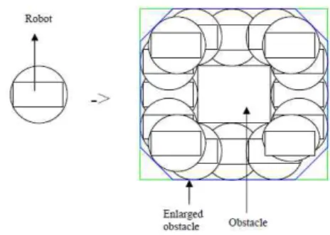
Fig. 1 Minkowski sum applied to the robot
path can be predefined taking into account information given but without considering random or unknown obstacles that may appear on the way to the goal. The same applies to completely known environments, but this topic is not covered in this paper as it is clearly less challenging.
To determine an optimal path in partially known environments, a combination of Minkowski Sum, VGR, Dijkstra’s algorithm, and a path smoothing algorithm that uses cardinal splines is utilised. Minkowski Sum provides a safe margin, the VGR generates all available paths, Dijkstra’s Algorithm is modified here to find the shortest path among the available paths generated using the VGR, and a path smoothing algorithm that employs the cardinal splines smooths the generated path such that the robot can physically follow the generated path.
In more detail, Minkowski Sum simplifies
the problem of a polygonal robot navigating
through obstacles by converting it to the
problem of a point object navigating through
enlarged obstacles instead. The obstacles are
enlarged, taking into account potentially the
worst case orientation of the robot in close
proximity of obstacles. For example, as
depicted in Fig. 1, the rectangular robot is
surrounded by a circle that is large enough
merely to cover the robot. The circle
subsequently traverses the edges of the
obstacle to generate the enlarged area of the
obstacle according to Minkowski Sum.
Fig. 2 Visibility graph representation and a modified version of Dijkstra’s Algorithm [9]
Fig. 3 Effect of tension in cardinal spline [8]
As depicted in Fig. 2, the VGR generates all available paths from the starting point (blue circle) to the goal (green circle). Dijkstra’s algorithm finds the shortest path amongst all the available paths as depicted in green in the same figure. Dijkstra’s algorithm is modified to find the path that is shortest in distance rather than in time. The original Dijkstra’s algorithm takes into account the number of turns that the robot needs to take before the robot reaches the goal. However, since the robot is assumed to travel at a low constant speed at this stage, the algorithm is modified to select the path that is shortest in distance instead.
Finally to smooth the generated path, a path smoothing algorithm that employs the concept of cardinal splines is utilised. For instance, if the path from A to E through B, C, and D in blue/dashed in Fig. 3 is an optimal path generated using the combined algorithm described above, then cardinal splines subsequently smooth the optimal path yielding the red path, which would be clearly easier for the robot to track. For further details on cardinal splines, readers are referred to [8].
Fig. 4 Robot structure
The combination of Minkowski Sum, VGR, Dijkstra's algorithm, and a path smoothing algorithm that uses the cardinal splines is referred to as KOA algorithm as previously mentioned. In partially known environments, unknown or random obstacles could also be present on the path that has been determined using the KOA algorithm. In such situations, the KOA algorithm is used alongside the ROA algorithm, reported in Section IV, to avoid both known and unknown (or random) obstacles.
Ⅲ. Basic navigation concepts
ROA algorithms allow robots to navigate without colliding with random or unknown obstacles. Before a ROA algorithm is introduced in the following section, this section describes the structure of the robot and sensors to allow the robot to avoid random obstacles. Mathematics (e.g. geometry) required for the robot equipped with sensors depicted in Fig. 4 to navigate around obstacles to reach the goal is also described. As depicted in the figure, the robot is assumed to be rectangular and includes a centre and front marker. The sensors A, B, C, and D (pentagons) provide a safety margin as indicated in blue/dashed.
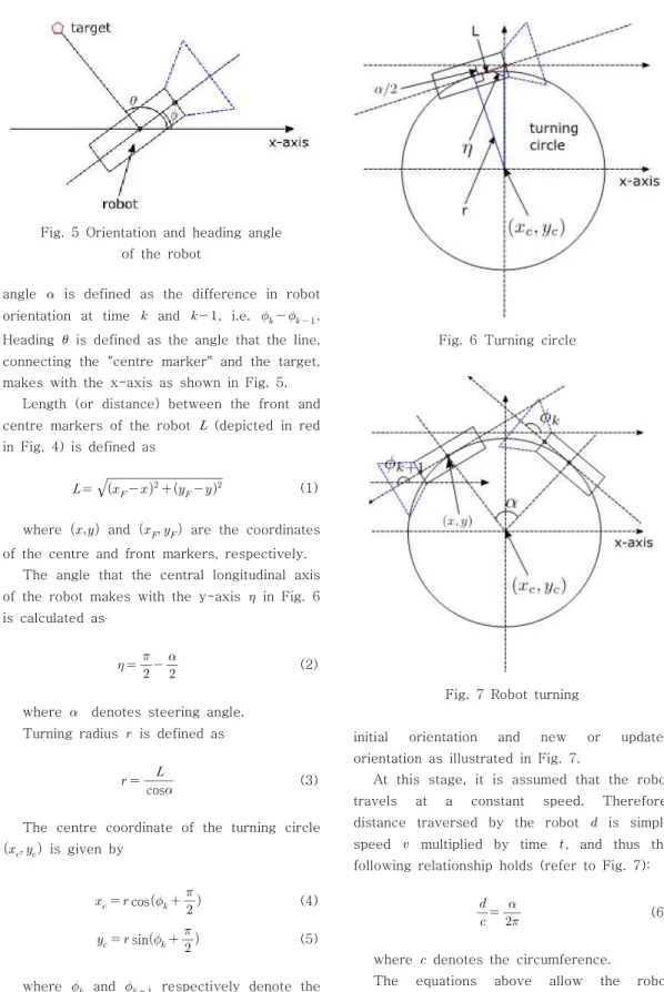
Orientation of the robot is defined as the
angle that the central longitudinal axis of the
robot makes with the x-axis as demonstrated
in Fig. 5. The robot depicted in Fig. 4 is
therefore at the orientation of (or initial
orientation). At any moment in time, steering
Fig. 5 Orientation and heading angle of the robot
angle is defined as the difference in robot orientation at time and , i.e.
. Heading is defined as the angle that the line, connecting the "centre marker" and the target, makes with the x-axis as shown in Fig. 5.
Length (or distance) between the front and centre markers of the robot (depicted in red in Fig. 4) is defined as
(1)
where and
are the coordinates of the centre and front markers, respectively.
The angle that the central longitudinal axis of the robot makes with the y-axis in Fig. 6 is calculated as
(2)
where denotes steering angle.
Turning radius is defined as
cos
(3)
The centre coordinate of the turning circle
is given by
cos
(4)
sin
(5)
where
and
respectively denote the
Fig. 6 Turning circle
Fig. 7 Robot turning
initial orientation and new or updated orientation as illustrated in Fig. 7.
At this stage, it is assumed that the robot travels at a constant speed. Therefore, distance traversed by the robot is simply speed multiplied by time , and thus the following relationship holds (refer to Fig. 7):
(6)
where denotes the circumference.
The equations above allow the robot
position after each time interval ∆ when steering angle is zero (i.e. the robot is moving straight) and when is nonzero to be calculated as follows [9]:
If
(7)
cos
(8)
sin
(9)
If ≠
(10)
cos
(11)
sin
(12)
In order to draw the robot at each time interval during simulation with the correct orientation, the following rotational matrix is employed.
cos
sin
sin
cos
(13)
where
is the initial position/coordinate of the robot's centre marker when
.
The following equations are employed to calculate heading with respect to obstacles, walls or the goal.
If ≥
cos
(14)
If
cos
(15)
where denotes the difference between the coordinates of the obstacle, walls or goal and the coordinate of the robot. denotes the length between robot centre and the obstacle, wall or goal.
The robot takes appropriate action when an obstacle or wall is detected within the safety
margin. As previously mentioned, it is assumed that there are 4 sensing points. Increasing the number of sensing points would improve the accuracy of the algorithm. However, it comes at the cost of increased computational effort, and 4 sensing points strikes a good balance between accuracy and simulation time at this stage.
Ⅳ. Random obstacle avoidance
Recall that cardinal spline is used for path smoothing in Section II. In this section, the concept of cardinal splines is exploited differently being part of the ROA algorithm as described in the following steps:
Step 1: Predetermine an optimal path In completely unknown environments, we assume that there is no obstacle present and find an optimal path which would simply be a straight line from the source (starting location) to the goal. In partially known environments, the algorithm introduced in Section II is employed instead to find an optimal path taking into account information given. This is demonstrated and simulated in Section V in more detail.
Step 2: Avoid obstacles on the path
While tracking the predefined path generated in Step 1, if the robot is faced with any random obstacles on the path, the robot steers away to clear the obstacles from the sensing range. The robot determines whether to turn right or left using the simple binary sensors A, B, C, and D shown in Fig. 3.
Moreover, if the robot encounters another obstacle when turning, then the sign of steering angle changes. Improvement as a result is demonstrated in the following section (in Fig. 11).
Step 3: Regenerate an optimal path
When an obstacle has been cleared, a new
optimal path is generated. It uses the concept
of cardinal splines illustrated in Fig. 3. The
control points are [A, A, B, C, D, E, E]
Fig. 8 Importance of the LAP
(a) Wrongly tuned
(b) Correctly tuned
Fig. 9 Importance of tuning the LAP
instead of [A, B, C, D, E] because A and E in [A, B, C, D, E] are only present to define the shapes of and , respectively, and the spline starts with B and ends with C. Using [A, A, B, C, D, E, E] instead, the first A and the last E are only present to determine the shapes of and , respectively, and the spline starts with the second A and ends with the second last E.
The control points for the cardinal splines for this study are thus [centre coordinates, centre coordinates, sensing point, look ahead point, goal, goal]. The Look Ahead Point (LAP) is important part of the ROA algorithm as explained below.
Step 4: Find a suitable LAP
Once an obstacle has been avoided, the objective now is to return to an optimal path.
To achieve this objective in a smooth manner, the LAP plays an important role. To find the
LAP, the closest point on the previously generated optimal path from the robot's current position needs to be found first. Subsequently, some distance towards the goal added to the closest point is known as the LAP. is a tuning factor that takes into account the sizes of the robot and obstacles and complexity of the sensing system used.
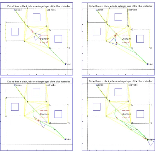
Fig. 10 Simulator with various examples
Fig. 11 Example 1, unknown environment (clockwise)
Fig. 12 Example 2, partially known environment (clockwise)
The importance of the LAP is illustrated in Fig. 8. In Fig. 8 (left), without the LAP the path is too sharp for the robot to follow. In Fig. 8 (right), the path is much smoother and easier for the robot to track due to presence of the LAP. This is the reason that the control points, [centre coordinates, centre coordinates, sensing point, LAP, goal, goal]), include the LAP. Note that the reason that "centre coordinates" and "goal" are included twice is explained in Step 3 above.
If the distance between the robot and goal is shorter than that between the robot and LAP, LAP is ignored to prevent the robot from deviating from its path unnecessarily.
The importance of tuning is illustrated in
Fig. 9(a) demonstrates a situation in which is too small causing the robot to orbit around the obstacle before it eventually reaches the goal.
In Fig. 9(b), is tuned correctly enabling the robot to reach the goal more smoothly and efficiently.
Ⅴ. Implementation and simulations
The algorithms developed in Sections Ⅲ and Ⅳ are tested in specially developed environments using the Graphical User Interface (GUI) in Matlab®. As depicted in Fig.
10, there are three different types of
environments to choose from on the left hand
side, namely, "Totally Known Environments",
Fig. 13 Example 3, partially known environment (clockwise)
"Partially Known Environments" and "Totally Unknown Environments". In each type, there are 4 different examples. One example from the Totally Unknown Environments and two examples from Partially Known Environments are presented here. The GUI with the initial screen when Example 4 from Partially Known Environments is selected is shown in Fig. 10.
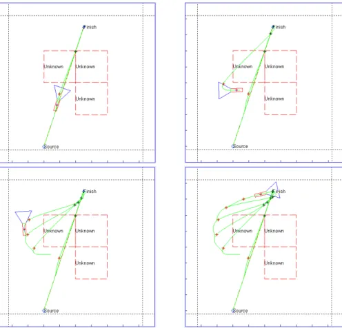
A totally unknown environment is presented in example 1. In the example (Fig. 11), there are three unknown obstacles (red/dashed), but no knowledge regarding the environment is provided in advance. As a result, only the ROA algorithm introduced in Section Ⅳ is employed and the KOA algorithm in Section III is not required. Since no knowledge of the environment is given the initial optimal path is
defined as a straight line from the starting point to the goal (or "Finish") as shown in the top left sub-figure. As shown in the following sub-figures (clockwise), it generates optimal paths 6 times to reach the goal. The regenerated paths and the corresponding LAPs are all displayed. It is important to note that when the robot encounters the first unknown obstacle, it turns left instead of right, thereby generating a more efficient path. This is due to the robot changing the sign of if the robot encounters another obstacle when turning as previously mentioned in Section Ⅳ (the last paragraph in Step 2).
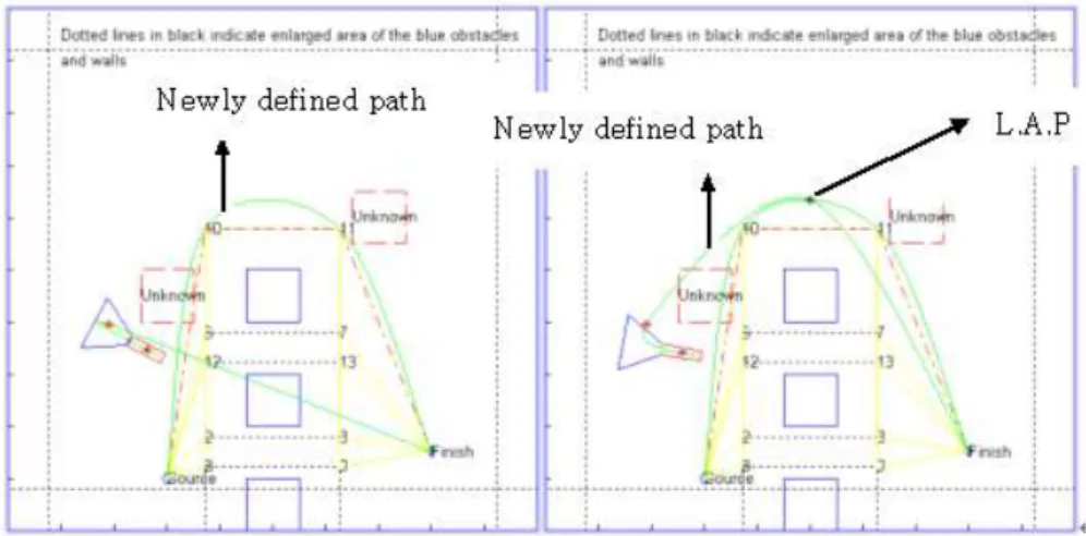
In the second example demonstrated in Fig.
12, both known and unknown obstacles exist;
that is, red/dashed and blue/solid rectangles
respectively depict unknown and known obstacles. The known obstacles are avoided by defining an optimal path as depicted in the figure, which is obtained using the KOA algorithm reported in Section Ⅱ. The green curve in the top left sub-figure is the optimal path and the yellow lines are the paths generated by the VGR while calculating the optimal path. To avoid the unknown obstacles (i.e. the two red/dashed rectangles), the ROA is also incorporated. All the paths that are generated during the simulation are displayed in the figure. It demonstrates that the robot successfully reaches the goal avoiding all the obstacles.
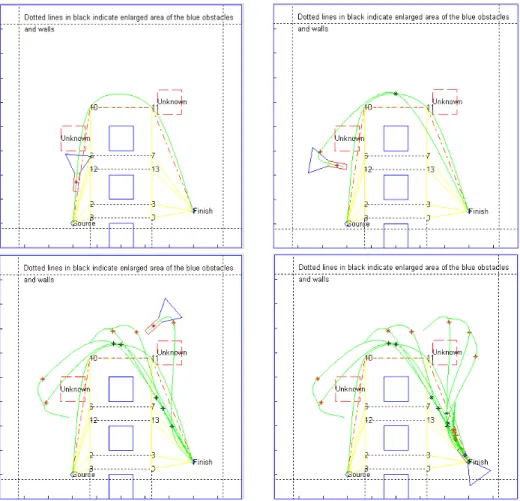
In example 3 (Fig. 13), similarly to example 2, an initial optimal path is first determined to avoid the known obstacles (three rectangles in blue/solid) using the KOA algorithm. While tracking the path, the robot encounters an unknown obstacle in red/dashed. The ROA algorithm is in turn activated and the robot avoids the unknown obstacle to reach the goal successfully.
Ⅵ. Conclusions
An efficient combination of Minkowski Sum, VGR, a modified version of Dijkstra's Algorithm, and a path smoothing algorithm that employs cardinal splines (i.e. KOA algorithm) is employed for predefining an optimal path given knowledge regarding the environments.
Moreover, a ROA algorithm to avoid random or unknown obstacles is reported. It breaks with the tradition and employs the concept of cardinal splines that use the LAP as one of the control points.
The simulation result in a totally unknown environment demonstrates that the ROA allows the robot to reach the goal without colliding into unknown obstacles. The simulation results in partially known environments illustrate that the ROA algorithm can be used successfully in addition to the KOA algorithm; that is, if the
robot encounters an unknown obstacle while following an optimal path defined using the KOA algorithm (for avoiding known obstacles), the ROA algorithm becomes active and enables the robot to avoid the unknown obstacle to reach the goal.
Taking into account the complexity of the proposed algorithms, the simulation results demonstrate that both the algorithms are efficient and the ROA algorithm is suitable for implementation on a small robot in which storage may be limited. For larger robots, this algorithm could serve as a useful basis for developing more sophisticated ROA algorithms.
Implementation of the proposed algorithms in a real-life small robot is reserved for future work.
References
[1] J. Craig, Introduction to Robotics : Mechanics and Control, 3rd Edition, Prentice-Hall, 2004.
[2] T. H. Cormen, C. E. Leiserson, R. L. Rivest, C. Stein, Introduction to Algorithms, 3rd Edition, MIT Press, 2009.
[3] M. D. Berg, M. V. Kreveld, M. Overmars, O.
Schwarzkopf, Computational Geometry, 2nd Edition, Springer-Verlag, 2000.
[4] J. O'Rourke, Computational Geometry in C, 2nd Edition, Cambridge University Press, 1994.
[5] K. Wu, T. Xi, H. Wang, “Real-time Three-dimensional Smooth Path Planning for Unmanned Aerial Vehicles in Completely Unknown Cluttered Environments,"
Proceedings of Region 10 Conference, pp.
2017-2022, 2017.
[6] A. C. Hildebrandt, M. Klischat, D. Wahrmann, R. Wittmann, F. Sygulla, P. Seiwald, D.
Rixen, T. Buschmann, “Real-Time Path Planning in Unknown Environments for Bipedal Robots," IEEE Robotics and Automation Letters, Vol. 2, No. 4, pp.
1856-1863, 2017.
[7] F. Kamil, T. Hong, W. Khaksar, M.
Moghrabiah, N. Zulkifli, S. Ahmad “New
Robot Navigation Algorithm for Arbitrary Unknown Dynamic Environments Based on Future Prediction and Priority Behavior,"
Expert Systems with Applications, Vol. 86, No. 15, pp. 274-291, 2017.
[8] I. J. Schoenberg, A. Sharma “Cardinal Interpolation and Spline Functions V. The
B-splines for Cardinal Hermit Interpolation,"
Linear Algebra and its Applications, Vol. 7, No. 1, pp. 1-42, 1973.
[9] O. Ringdahl, “Path Tracking And Obstacle Voidance Algorithms for Autonomous Forest Machines," Master's thesis, Umea University, 2003.
Sung-ho Hur (허 성 호)
He received the B.Eng.
degree in Electronics and Electrical Engineering from the University of Glasgow, UK in 2004, the M.Sc. degree (with Distinction) in Electronic and Electrical Engineering from University of Strathclyde, UK in 2005, and the Ph.D. degree with in Control (within the department of Electronic and Electrical Engineering) from University of Strathclyde (2006-2010).
He is now an Assistant Professor, within the School of Electronics Engineering at Kyungpook National University.
His research interests include control, wind energy, obstacle avoidance, and cross-directional process.
Email: [email protected]
![Fig. 2 Visibility graph representation and a modified version of Dijkstra’s Algorithm [9]](https://thumb-ap.123doks.com/thumbv2/123dokinfo/5339047.393897/3.772.427.677.134.305/fig-visibility-graph-representation-modified-version-dijkstra-algorithm.webp)