Methodology of Spatio-temporal Matching for Constructing an Analysis Database Based on Different Types of Public Data
10
0
0
전체 글
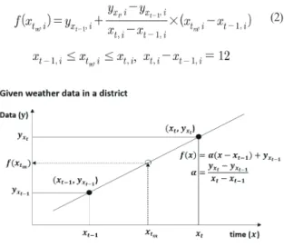
(2)
(3)
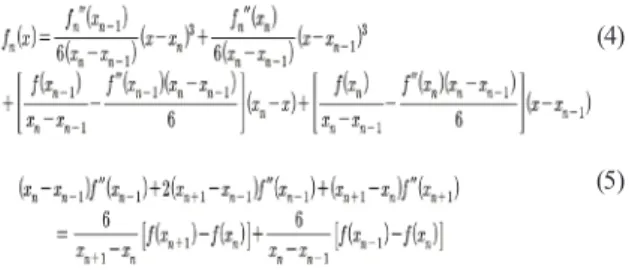
(4)
(5)
(7)
(8)
(9)
(10)
수치
+3
관련 문서