Prediction of the Major Factors for the Analysis of the Erosion Effect on Atomic Oxygen in LEO Satellite Using a Machine Learning Method (LSTM)

Vol.14, No.2, pp.50-56 (2020)

Prediction of the Major Factors for the Analysis of the Erosion Effect on Atomic Oxygen in LEO Satellite Using a Machine Learning Method (LSTM)

You Gwang Kim

, Eung Sik Park

, Byung Chun Kim

, Suk Hoon Lee

and Seo Hyun Lee

1

Korea Aerospace Research Institute

2

National Institute for Mathematical Sciences

3

Insight Mining

Abstract

In this study, we investigated whether long short-term memory (LSTM) can be used in the future to predict F10.7 index data; the F10.7 index is a space environment factor affecting atomic oxygen erosion. Based on this, we compared the prediction performances of LSTM, the Autoregressive integrated moving average (ARIMA) model (which is a traditional statistical prediction model), and the similar pattern searching method used for long-term prediction. The LSTM model yielded superior results compared to the other techniques in the prediction period starting from the max/min points, but presented inferior results in the prediction period including the inflection points. It was found that efficient learning was not achieved, owing to the lack of currently available learning data in the prediction period including the maximum points. To overcome this, we proposed a method to increase the size of the learning samples using the sunspot data and to upgrade the LSTM model.

Key Words : Machine Learning, LSTM, ARIMA, Atomic Oxygen, Erosion, Factor Forecasting, Statistical Method, LEO

XXUUGGpp••››™™––‹‹œœŠŠ››––••GG

Recently, convergence research on technologies utilizing artificial intelligence (AI) and big data in various fields has drawn significant attention. In relation to this trend of convergence research, there has been an increasing interest in the optimized design of low-Earth-orbit (LEO) satellites.

Moreover, there was a recent report of a study using statistical techniques to predict the atomic oxygen erosion in satellite coating materials considering the effects of the space environment under the worst-scenario condition [1]. In this study, among the major factors related to the space environment affecting the erosion of the coating materials of LEO satellites by atomic oxygen, the index data of F10.7, which is a solar radio flux, were predicted. This was conducted by applying mathematical and statistical techniques used for big data analysis and machine learning. Based on the results, we aim to present a methodology that can be useful for determining the coating material thickness in satellite design in the future.

An LEO satellite is designed to perform its mission even when exposed to an unfavorable space environment, which is very different from the ground condition. Among the design

considerations, the erosion of polymer materials by the atomic oxygen species distributed in the low orbits of the Earth is a phenomenon not observed on the ground. These atomic oxygen species collide with the exterior of a satellite at a speed of approximately 7.8 km/s, which corresponds to the orbital speed of a low-orbiting satellite, resulting in the problem of degradation of the properties of the coating material [2]. The coating material of satellite parts is designed considering the various effects of the space environment;

however, the design of the protection against the atomic oxygen erosion employs a robust method [1] assuming the worst-case scenario. In this study, we aimed to present a basis for more realistic prediction-oriented design based on existing measurement data by mathematical/statistical techniques.

YYUUGGww™™ŒŒ‹‹ŠŠ››––••GG” ”ŒŒ››––‹‹GG

Research on atomic oxygen erosion-related detailed technologies and prediction techniques has not been extensively reported or published worldwide, and even the advanced countries in the field of space sciences do not share technical details. Therefore, satellite designs in Korea, until recently, were based on a robust design that simply assumed the worst-case scenario. In our previous study [1], we aimed to establish an F10.7 prediction model by applying various Received: Jan. 13, 2020 Revised: Mar. 17, 2020 Accepted: Apr. 01, 2020

† Corresponding Author

Tel: +82-42-860-2535, E-mail: [email protected]

Ⓒ The Society for Aerospace System Engineering

mathematical and statistical techniques as a manner of trial and error, and focused on techniques producing small errors.

In this study, our objective was to predict highly detailed F10.7 data during the mission period. The F10.7 index is a necessary input variable for the calculation of atomic oxygen erosion using long short-term memory (LSTM) among the machine learning techniques that have rapidly developed in recent years. This is based on the analysis of the F10.7 data measured and published internationally.

This study focused on the prediction of F10.7 data; F10.7 is an important space environment factor in the calculation of atomic oxygen erosion during a satellite mission. In the future, we aim to further develop these mathematical and statistical prediction models, so that the results can actually be used for the calculation of atomic oxygen erosion of the satellite materials. However, such a research is considered to require additional experiments and cost as well as significant time consumption. Therefore, to organize the research outputs in a stepwise manner, first, we investigated the F10.7 data prediction method.

YYUUXXGGuuŒŒŠŠŒŒšššš››  GG––GG——™™ŒŒ‹‹ŠŠ››––••GG

The F10.7 and Ap indices, which are important factors in the space environment for the prediction of atomic oxygen erosion, serve as indicators related to solar activity and are affected by the solar cycle or solar magnetic activity cycle. Solar magnetic activity has been reported to change with a cycle of approximately 11.1 years. This change depends on the solar activities (including changes in the level of solar radiation and material ejection from the sun) and variation in the solar appearance (such as changes in the number of sunspots and size, flares, and other signs). These changes in the solar magnetic activities affect the atmosphere and the surface of the earth periodically or aperiodically.

Fig. 1 Forecasted Solar Cycle 25 (NOAA/NASA) [3]

The data released on December 9, 2019 by the Space Weather Prediction Center jointly hosted by National Oceanic and Atmospheric Administration(NOAA)/National Aeronautics and Space Administration(NASA) is shown in Fig. 1. According to it, Solar Cycle 25 has the highest point in July 2025 (± 8 months) and the lowest point in April 2020 (± 6 months), and the expected highest sunspot number (smoothed sunspot number (SSN)) is 115, which is expected to be similar to Solar Cycle 24 [3].

The prediction of the F10.7 value is necessary for the estimation of atomic oxygen erosion during the planned mission period of a satellite from the point of its launch, and the data analysis in a previous study [1] reported the periodicity and pattern in the data. Therefore, optimization of the design of the polymer materials considering atomic oxygen erosion was considered necessary.

YYUUYYGGk kˆˆ››ˆˆ G

As is known from numerous space environment studies, solar activity is an important factor in the space environment;

it has the largest effect on the atomic oxygen erosion of LEO satellite coating materials. The indices representing these solar activities are expressed in a variety of forms in each field.

However, among the indicators related to solar activity, the input variables used in the prediction calculation of the atomic oxygen erosion of an LEO are the solar radio flux (F10.7) and geomagnetic index (Ap) values provided by the SPace ENVironment Information System (SPENVIS) of the European Space Agency (ESA) [2].

The F10.7 index is known to be the most classical value in the methods for directly recording solar activity, besides those related to sunspots. F10.7 is a measure of the solar flux per unit frequency at a wavelength of 10.7 cm near the high point of the observed solar radiation. It is represented as the size of the 2,800-MHZ (10.7-cm) radio flux measured by day per solar flux unit (SFU) (1 × 10

W m

Hz

).

The Ap index is a measure of the mean daily level of the geomagnetic activity on the Earth during the corresponding one day of universal time (UT). Moreover, the values measured at various locations worldwide, for the change in the magnetic field of the Earth due to the current flowing through the ionosphere of the Earth, are determined at the GeoForschungsZentrum (GFZ) Institute in Potsdam, Germany.

Furthermore, they are presented on behalf of the International Service of Geomagnetic Indices (ISGI) of the International Association of Geomagnetism and Aeronomy (IAGA).

In this study, as described above, from the two important indices affecting the atomic oxygen erosion of a LEO satellite coating material, a prediction of the F10.7 index with periodicity was performed. Compared to the F10.7 index, the Ap index is known to have a weak periodicity or regularity in the pattern (the correlation coefficient between the Ap Index and SSN, which is a representative index of the solar activity, is reported as 0.32.). Moreover, because this change occurs irregularly, this index shows no difference depending on the technique used. Therefore, in this study, improving the existing prediction method of the Ap index was not considered.

YYUUZZGGww™™ŒŒ‹‹ŠŠ››––••GG››ˆˆ™™ŽŽŒŒ››GG——ŒŒ™™––‹‹GG

Assuming that the mission period of a satellite is 5 years

and the preparation period is 2 years, the period for the next 7

years from the present should be predicted considering these

periods. The actual data available under these assumptions are

up to 7 years before the launch date. Therefore, this study

predicted F10.7 over the next 7 years from a planned satellite

launch time, including a preparation period of 2 years and a

mission period of 5 years. Moreover, it was assumed that

among the currently collected data, there are no data for the recent 7 years, and the prediction was performed under this assumption. Following the prediction, the results were compared with real data, and the prediction performance was evaluated.

With regard to these assumptions, the mean design period of the satellites developed in Korea is typically approximately 5 years; therefore, adding 5 years of the mission period will require more than 10 years in total. Despite this, the satellite development period and mission periods were set as 2 years and 5 years, respectively. This was because the critical design review (CDR) of the Korea Multipurpose Satellite (KOMPSAT), which is a type of LEO satellite, was conducted 2–2.5 years before its launch. The final details of the design are confirmed at this CDR stage; therefore, the development period was set as 2 years. As for the mission period, those of the KOMPSAT or the next-generation middle-sized satellites are typically set as 3.5–5 years. Therefore, considering a buffer time of margin, it was considered that the prediction of the atomic oxygen erosion should be reflected in the design at least 7 years before the actual design work. Based on the start time of an actual satellite design, the design period of 2 years is not realistic. However, because the Korea Aerospace Research Institute (KARI) has numerous design heritages of the KOMPSAT program, the maximum period of the prediction was set as 7 years, to improve the prediction accuracy of the atomic oxygen erosion. (Specifically, it is empirically recognized that predicting for a period of 10 years or more is to some extent less accurate.)

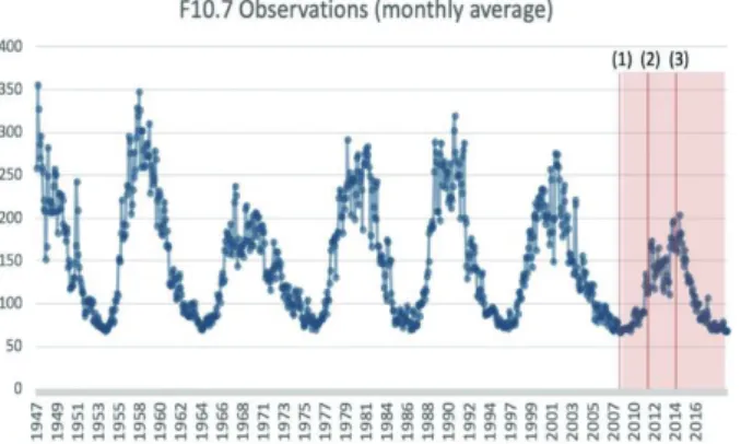
Because the collected F10.7 data [4] were for the period from March 1947 to July 2019, the data used for the prediction were the data excluding those from the most recent time point to July 2012, excluding the period of the past 7 years. Using this, we predicted the F10.7 values for the next 7 years, and compared the predicted values with the actual F10.7 values.

The evaluation of the predicted value was performed using a five-year prediction error from August 2014 to July 2019, assuming that the period was the time for the actual mission period, excluding the preparation period.

Fig. 2 F10.7 Monthly Averaged Data

Concurrently, when analyzing the past observation data presented in Fig. 2, the forecast period, from August 2014 to

July 2019, appears as a descending period from maximum to minimum in the cycle of the F10.7 index. To consider the effect of the period characteristics in a cyclic process, the predictions at the point with the increase from the minimum to the maximum and the midpoint of the descending from the maximum to minimum were added to compare the results.

Based on the graph of the F10.7 index, the period with the increase from the minimum to the maximum was from August 2008 to July 2013. Moreover, the period that starts from the midpoint of the rise from the minimum to the maximum, which includes the maximum point, was August 2011 to July 2016, and the starting points of the prediction are displayed in Fig. 2, where they are denoted as (1), (2), and (3)

ZZUUGGhh————““ŠŠˆˆ››––••GG––GGww™™ŒŒ‹‹ŠŠ››––••GGt tŒŒ››––‹‹GG

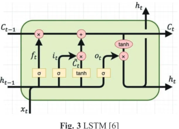
In this study, we applied the LSTM technique, which has been recently reported to present good performance as a machine learning technique for time series data. The results were compared to those of the autoregressive integrated moving average model (ARIMA), which is a representative statistical methodology for processing time series data.

Another comparison was performed with the results of a similar pattern searching method proposed in a previous study.

As a parameter for comparing predictive performance, a prediction error, which is the difference between the predicted and actually measured and internationally published F10.7 values, was used. As for the calculation of the prediction error, the root mean squared error (RMSE) and the mean absolute percentage error (MAPE) were used. The RMSE was obtained by averaging the square of the difference between the predicted and actual measured value. The MAPE was obtained by taking the mean value of the calculation of the percentage of the absolute value of the difference between the predicted and actual measured values divided by the actual value. The calculation formulas are given below.

RMSE = √

^{and (1)}

MAPE =

|𝑦𝑦̂𝑡𝑡+ℎ−𝑦𝑦𝑡𝑡+ℎ|

𝑦𝑦𝑡𝑡+ℎ ×100) 𝑛𝑛ℎ=1

𝑛𝑛

, (2)

where

𝑦𝑦̂

: Prediction value

𝑦𝑦

: Observation value

n : Number of samples

It can be inferred that the smaller the RMSE and MAPE, the better the performance of prediction. The prediction error was calculated from the three prediction target periods, which were from August 2014 to July 2019, August 2011 to July 2016, and August 2008 to August 2013. For these periods, the predicted and actual measured values of the F10.7 index were used for the calculation of the error.

ZZUUXXGGss––••ŽŽGGzz––™™››TT{{ŒŒ™™” ”GGt tŒŒ” ”––™™  GGOOsszz{{t tPPGG››ŒŒŠŠ••˜˜œœŒŒGG LSTM is a model proposed by Hochreiter et al. (1997). It is a machine learning algorithm appropriate for processing sequential data, such as time series data, and has recently presented good performance in various fields related to big data.

Fig. 3 LSTM [6]

To be more specific regarding the description, LSTM is a type of artificial neural network with a cyclic structure, and it was designed to overcome the vanishing gradient problem, for which recurrent neural networks (RNNs) become gradually less effective for adjustment as the steps progress [5]. As shown in Fig. 3, the key concept is a network structure including three gates: a forget gate that maintains the appropriate level of past information and then completely forgets it, an input gate that controls the memory level of the current information, and an output gate that produces the final result. Through the forget gate, data and information from the past are appropriately preserved in the network, so that they continue to have an effect on prediction of the future values.

Owing to this structural advantage, LSTM is a very extensively used deep learning method for time series prediction.

In this study, as displayed in Fig. 4, a model was established to minimize the error in predicting the F10.7 data for the next month from the observations of 30 consecutive months, i.e., the 31

month. This method implemented trial and error processes of 15 months, 30 months, and 45 months, minimizing the error to derive the optimum value. Therefore, from this model, the August 2012 value was predicted from

the observations from February 2010 to July 2012. Moreover, using the observed values from March 2010 to July 2012 and the predicted value of August 2012 in the previous step, the value of the next month, September 2012, was predicted. This method was applied consecutively to calculate the prediction values up to July 2019

Fig. 4 LSTM Prediction by Trial and Error Also, before the learning process began, as for the hyper- parameter values used, 9 learning rates were set between the values from 0.1 to 0.001. The early stopping rule was applied in which the learning rate was lowered whenever the learning was stopped and for each learning rate, an epoch of 2000 times was set, and when there was no progress, it moved on to the next step.

ZZUUYYGGhhœœ››––™™ŒŒŽŽ™™ŒŒššššŒŒGG••››ŒŒŽŽ™™ˆˆ››ŒŒ‹‹GG” ”––••ŽŽGGˆˆŒŒ™™ˆˆŽŽŒŒGG OOhhyyppt thhPPGG” ”––‹‹ŒŒ““ GG

ARIMA a most widely used methodology when analyzing time series data and making predictions using models [7].

Fig. 5 ARIMA Equation [7]

The essence of the ARIMA model is an analysis technique

that generalizes an auto-regressive moving average (ARIMA)

model that describes the current time series values using past

observations and errors. However, the model can be applied

only to stationary series, which is a time series. Specifically,

the mean and the variance do not change regardless of the

trend of time, and the covariance between the time points is

not affected by the reference point. In the prediction model

used, as presented in Fig. 5, a prediction value at a certain time point is assumed as a linear combination of p observed values and q errors that occurred in the past. The prediction process consists of three stages as follows: a stage identifying p and q, the required parameters in this model; a stage of estimating the coefficients according to the selected p and q; and a stage of diagnosing the model.

However, a non-stationary time series with periodicity as well as high and low maximum point values, is transformed into a stationary time series by a variable transformation, such as logarithmic transformation and difference, and then the identification and estimation and the diagnosis processes for the model are performed. In this case, both the difference between the neighboring time points and the seasonal difference to solve the fluctuations occurring in the cycle are identified, and the model in this case is called ARIMA. In this study, a logarithmic transformation was performed to convert the series into a stationary series, and the difference was set as 1. The seasonal difference was set as 130 months, because the F10.7 index presents similar patterns to the solar activity cycle.

Moreover, as the final model, ARIMA (1,1,5) × (1,1,2)

was applied, based on the autocorrelation and partial autocorrelation functions.

ZZUUZZGGzz” ”““ˆˆ™™GG——ˆˆ››››ŒŒ™™••GGššŒŒˆˆ™™ŠŠ••ŽŽGG

The similar pattern searching technique is a very realistic technique proposed in a previous study [1].

Fig. 6 F10.7 Prediction Concept using Similar pattern The specific methodology of the technique is illustrated in the following example. As depicted in Fig. 6, taking the period from the most recent point to 7 years ago as a reference in the data used in the prediction, the period most similar to this period is searched for from the past data. Moreover, the data of the next 7 years after the most similar period are used as the prediction values. For example, when the prediction starts from August 2012, the periods that are most similar to the data for the 7 years from August 2005 to July 2012 are searched for

from the collected past data. Here, “similar period” is selected as the period having the smallest sum of the squared errors with the F10.7 value of the reference period (set as “mission period” here). For the given data, the F10.7 data from December 1960 to November 1967 are chosen as the most similar period.

Therefore, excluding the preparation period, the prediction values for the period most similar to the mission period from August 2014 to July 2019 is regarded as the data from December 1969 to November 1974.

ZZUU[[GG Comparison of characteristics between prediction techniques GG

As described above, the ARIMA model is developed based on the strong assumption of a linear combination of the past observations and errors and the assumption that the time series data should be stationary. Therefore, it is efficient for a short- term prediction in case the assumption is satisfied. However, as the prediction period becomes longer, it tends to converge to the mean value and has the disadvantage of the confidence interval becoming large.

Concurrently, the similar pattern searching method, which is a data-driven technique without using any model, has the advantage that it does not use a model unlike ARIMA or LSTM. However, in the results of searching for a period in the past similar to the recent 7 years, there was a problem in that several candidate similar periods with similar differences were found, and there was a disadvantage that the confidence interval could not be obtained.

Contrastingly, the ARIMA model makes a strong assumption of a stationary state and a linear model, whereas because LSTM is a non-linear model, if the optimization is effective, prediction values with smaller errors than in the ARIMA method can be obtained. However, this method also has a problem of over-fitting, which is typical for non-linear models. Furthermore, another problem is that in the case when there are numerous cases of selecting hyper-parameters that need to be input depending on the characteristics of the data applied, the optimization relies on a trial and error methodology.

[[UUGGww™™ŒŒ‹‹ŠŠ››––••GGyyŒŒššœœ““››ššGG

[[UUXXGG Prediction results for the period from August 2014 to July 2019 GG

In Fig. 7, the comparison of the predicted and actual observed data for the period from August 2014 to July 2019 by applying the three proposed methods (LSTM, ARIMA, and similar pattern searching method) is shown.

From the prediction results of the three methods, it is found

that LSTM reflects realistic change patterns for the period

from 2014 to 2019 more than the other two methods, and the

similar pattern searching method is the next best. For the ARIMA method, as described in the previous section of comparing the characteristics of the prediction methods, the applied model tends to converge to a mean value in the case of long-term prediction; this model reflects almost no changes.

Regarding the level of errors comparison, as listed in Table 1, the RMSE is 19.19 and MAPE is 16.08 for LSTM, which are relatively small compared to those of the other two methods, indicating that its performance is superior to those of the other methods.

Fig. 7 Prediction of F10.7 Using Three Models [[UUYYGGjj––” ”——ˆˆ™™šš––••GG––GG››ŒŒGG——™™ŒŒ‹‹ŠŠ››––••GG——ŒŒ™™––‹‹ššGG

The above prediction period comparison from August 2014 to July 2019 is a comparison of the case of descending from the maximum point to the minimum point in this period.

In this part of the study, to investigate whether the prediction method is affected by the change in the patterns of the prediction target period, two additional prediction periods were considered. These are from August 2011 to July 2016 (which is the period starting from the midpoint of the rising from the minimum point to the maximum point) and from August 2008 to July 2013 (a period rising from a minimum point to the maximum point). The results are summarized in Table 1

Table 1 Performance Comparison of Predictions LSTM ARIMA Similar Pattern

RMSE

2014.8–2019.7 (maximum point→minimum

point)

19.19 43.27 39.46

2011.8–2016.7 (period including

maximum points) 99.82 53.43 80.39

2008.8–2013.7 (minimum point→maximum

point)

65.71 88.57 79.65

MAPE

2014.8–2019.7 (maximum point→minimum

point)

16.08 36.10 38.25

2011.8–2016.7 (period including

maximum points) 59.02 26.63 48.73 2008.8–2013.7

(minimum point→maximum

point)

52.50 76.89 59.24

LSTM presents a smaller error than the other two methods in the two prediction periods from the maximum to the minimum and from the minimum to the maximum However, the largest error is found in the period including the maximum point starting from the midpoint of the minimum point and the maximum point. The fact that LSTM yields the smallest error in the two prediction periods indicates that the model is considerably accurate when estimating the period from a given period of data. However, in the period including the maximum point, the model showed the largest error. The reason that the learning was not performed well in LSTM in this period is that in the observed values from 1947 to 2008, there are 6 occurrences of maximum points, and one of the maximum point periods has different characteristics from those of the other 5 maximum point periods, making the learning difficult for the model. This characteristic is similar to that of the results of the similar pattern searching method, which considers the change pattern of the entire period.

These results correspond to 49.66% for LSTM, 34.17% for ARIMA, and 60.35% for the similar pattern searching method, compared to the F10.7 value of 250, which is applied as a constant in the past robust design values. In the robust design in the past, a constant value used for F10.7, and 250 is an overfitted value by approximately 52.85% compared to 117.88, the mean value of the F10.7 data in the period. Therefore, the predicted values, when compared to the mean value of the F10.7 data that were actually measured, are 5.32% for LSTM, –27.52% for ARIMA, and 28.0% for the similar pattern searching. Here, (+) indicates the value is predicted to be higher than the actual value and (-) indicates that the value is predicted to be lower than the actual value .

\\UUGGjj––••ŠŠ““œœšš––••GGˆˆ••‹‹GGmmœœ››œœ™™ŒŒGGyyŒŒššŒŒˆˆ™™ŠŠGGn n––ˆˆ““ššGG

Because the tests in real space environments (e.g.,

experiments of material exposure under the space environment

at the International Space Station) are extremely difficult to be

conducted in practice, studies that simulate or predict space

environments are needed [8]. This study was started with the

aim of providing a foundation for the convergence research

between various institutions. As the first goal, this study aimed

to optimize the design of satellite polymer materials, including atomic oxygen erosion calculations. Based on this, we intend to develop the research into a cross-organizational study related to the analysis and prediction of national space data utilizing machine learning techniques.

In this study, as a prediction technique of the F10.7 index, which is an important factor affecting atomic oxygen erosion in the space environment, we aimed to verify the applicability of LSTM, a machine learning technique that is actively used for time series data analysis. The results of the comparative analysis of the prediction performance of the ARIMA model, a conventional time series data analysis model proposed in the previous study, and the similar pattern searching technique were derived, and finally, the applicability of the LSTM method was confirmed.

As presented by the study results, the LSTM method, with an accurate prediction of the cycle, was more accurate in terms of the size of the error compared to the traditional method, ARIMA. However, when predicting the section containing the maximum points, owing to the limitation in the given data, LSTM had a larger error than the ARIMA method. Therefore, to improve this prediction error, larger learning data are required. In this regard, the additional utilization of sunspots data, which are known to have a large correlation with the F10.7 index and the improvement of the LSTM model to better train the change, are considered as possible future research. When the mathematical and statistical prediction models proposed in this study are improved and used, they are expected to improve the accuracy of the prediction of the atomic oxygen erosion of the polymer materials used in space for the development of LEO satellites. This knowledge will be transferred to the private sector in the future, and it is also expected to bring practical benefits in terms of efficiency and cost-effectiveness in the optimization design and manufacturing process of such satellites in the future.

yyŒŒŒŒ™™ŒŒ••ŠŠŒŒššGG

[1] Y. G. Kim, E. S. Park, B. C. Kim, S. H Lee, and S. H. Lee,

“The case study on the optimized forecasting methods of major factors for the analysis of the atomic oxygen erosion effect in LEO satellite,” Proc. of KSAS 2019 Fall Conference, Cheju, Korea, pp. 203, November 2019.

[2] www.spenvis.oma.be.

[3] https://www.swpc.noaa.gov/news/solar-cycle-25-forecast- update, Dec. 09, 2019.

[4] ftp://ftp.geolab.nrcan.gc.ca/data/solar_flux/daily_flux_

values/.

[5] S. Hochreiter and J. Schmidhuber, “Long short-term memory,” Neural Computation, vol. 9, no. 8, pp. 1735- 1780, 1997.

[6] S.-K. Park, “Principle and formula calculation of LSTM,”

http://docs.likejazz.com/lstm/, May 30, 2018.

[7] M. Mishra, “Unboxing ARIMA models,” https://towards datascience.com/unboxing-arima-models-1dc09d2746f8, Jun 11, 2018.

[8] Y. G. Kim, S. T. Lee, M. J. Baek, and S. H. Lee,

“Prediction of atomic oxygen erosion for coating material

of LEO satellite’s solar array by using the real RAM

direction accumulation method,” Journal of Aerospace

System Engineering, vol. 11, no. 5, pp. 1-5, 2017.