Analysis of residential natural gas consumption distribution Analysis of residential natural gas consumption distribution Analysis of residential natural gas consumption distribution Analysis of residential natural gas consumption distribution
function in Korea - a mixture model function in Korea - a mixture model function in Korea - a mixture model function in Korea - a mixture model
Ho-Young Kim, Seul-Ye Lim, and Seung-Hoon Yoo
Department of Energy Policy, Graduate School of Energy & Environment, Seoul National University of Science & Technology
(Received 4 August 2014, Revised 15 September 2014, Accepted 17 September 2014) Abstract
The world’s overall need for natural gas (NG) has been growing up fast, especially in the residential sector.
The better the estimation of residential NG consumption (RNGC) distribution, the better decision-making for a residential NG policy such as pricing, demand estimation, management options and so on. Approximating the distribution of RNGC is complicated by zero observations in the sample. To deal with the zero observations by allowing a point mass at zero, a mixture model of RNGC distributions is proposed and applied. The RNGC distribution is specified as a mixture of two distributions, one with a point mass at zero and the other with full support on the positive half of the real line. The model is empirically verified for household RNGC survey data collected in Korea. The mixture model can easily capture the common bimodality feature of the RNGC distribution. In addition, when covariates were added to the model, it was found that the probability that a household has non-expenditure significantly varies with some variables. Finally, the goodness-of-fit test suggests that the data are well represented by the mixture model.
Key words : residential natural gas consumption, zero observations, mixture model, distribution function, Weibull distribution
서 론 1.
The world’s overall need for natural gas (NG) has been growing up fast. Global demand for NG has risen steadily for the past several decades, and this trend appears to continue. One reason is price, and other reasons are fuel diversification, energy security issues, economic growth, and environmental concerns. NG is a very versatile fuel that can be used for space and water heating, processing heat for industry, electricity generation, cooking, mechanical power and transportation (Lim and Yoo 2012). For these various purpose of NG use, NG consumption in many countries has been
increasing (BP 2012).
Over the last two decades, the NG consumption in Korea has increased at a high annual growth rate of 18.7 percent (Yoo et al. 2009). This is due to the expansion of the infrastructure for gas distribution and an increase in individual income.
Crucial factors that underlie the recent rise in the consumption of NG have been an upsurge in the urban NG consumption and an increase of fifty five percent in the proportion of the urban NG consumption of gas that occurs in the residential sector. A significant number of households have switched from oil and coal to NG and electricity in Korea. The NG consumption has increased dramatically since natural gas began to be supplied in 1987. Thus, NG is the main source of energy for households in urban areas, accounting for fifty five percent of the residential consumption of energy.
http://dx.doi.org/10.5855/ENERGY.2014.23.3.036
To whom corresponding should be addressed.
Department of Energy Policy, Graduate School of Energy &
Environment, Seoul National University of Science & Technology Tel : 02-970-6802 E-mail : [email protected]
However, Korea has scarce reserves of NG, which is therefore imported entirely from NG-producing countries. The supply chain for NG in urban areas in Korea is structured as follows.
NG is imported in the form of liquefied NG (LNG) from foreign countries and is then supplied to domestic gas companies (wholesale companies and a monopolized public utilities company that is owned by the Korean government). It is also supplied to regular, urban, gas companies (for-profit retail companies and private firms) that supply to households, businesses, and industries.
Thus, the consumer’s price for urban gas is comprised of the cost of importation and the wholesale and retail firms’ expenses for supplying gas. Among the various components of cost, the cost of importation fluctuates due to fluctuations in the international price of oil and the exchange rate.
Being public fees, the expenses of wholesale and retail firms are regulated by local governments and legislative assemblies. The central and local governments suppress price increases by lowering and freezing fees.
On the other hand, the international price of LNG has recently been at a very high level due to the high price of oil. The high price of oil aside, the actual prices of goods are higher than ever before due to the impact of technological and seasonal factors upon the short-term supply and demand for NG. In particular, the price levels, which in the past several years showed a downward trend, are now showing an upward trend, as per a recently concluded long-term contract. This reverse trend is due to an increase in demand, increased uncertainty in the ability to increase supply, and the expectation that the price of oil will remain high, besides various other interdependent factors.
Therefore, the international LNG market is expected to be unfavorable to LNG-importing countries such as Korea. In this context, to balance supply with demand, the demand or consumption for NG needs to be accurately analyzed and predicted, especially for the residential sector. This
can be achieved by analyzing the pattern of residential NG consumption (RNGC). In addition, the estimation of the RNGC distribution function will provide useful information for pricing-related policies relating to importation and the costs of supply.
Many studies have been conducted on the estimation of the residential demand function for NG (Bernddt and Watkins 1977; Bloch 1980;
Blattenberger et al. 1983; Balestra and Nerlove 1996). However, to the best of the author’s knowledge, investigations of the RNGC distribution function are not available. RNGC distribution is the basis for the decision-making about pricing, demand estimation, management options and so on. The better the estimation of this distribution, the better decision-making for a residential NG policy. The RNGC distribution is a crucial information in planning a NG project and detailed knowledge of the RNGC is needed to estimate the performance of a NG project.
Therefore, this paper attempts to approximate the RNGC distribution function using a specific case study of Korea. To gather data, a survey of households was conducted in Korea. A typical observation in the consumption survey is that many households tend to give zero responses. Zero consumption of a good may arise as a corner solution of the consumers’ utility-maximization when the good does not contribute at all to the individual’s utility or is so remote from his or her interest that he or she is completely indifferent to it.
One example is the household RNGC. About seventeen per cent of all households reported zero RNGC, as will be explained in Section 3.
Thus, approximating RNGC distribution should consider the fact that some households do not spend at all on NG. In other words, the RNGC distribution tends to be bimodal. This complicates the approximation. In this case, a more flexible specification of the RNGC distribution is required.
One of the possibilities of allowing for the bimodality is to use a mixture model (McLachlan
and Basford 1988; Yoo 2004). The mixture model incorporates the possibility of an individual’s RNGC being zero. The purpose of this paper, therefore, is to apply a mixture model to approximation of RNGC distribution in order to capture the bimodality. The RNGC distribution is specified as a mixture of two distributions, that is, one with a point mass at zero and the other with full support on the positive half of the real line.
Moreover, the mixture model is estimated without and with some covariates, and a goodness-of-fit test is then performed for the model.
2. The model
The mixture model applied here can be interpreted as the mixture of two distributions, which incorporates not only positive but also zero RNGC responses. One can recognize that RNGC level (hereinafter denoted as ) is a random variable with the probability density function (pdf) and the cumulative distribution function (cdf), defined here as and , respectively, where is a vector of parameters. Let us assume the pdf of the RNGC to have the following form:
i f
i f
i f (1) where is an absolutely continuous pdf defined over positive real line. Thus, the cdf of the RNGC takes the form:
for ≥ (2) where is an absolutely continuous cdf such that . As can be seen from equation (2), is not absolutely continuous. It has a point mass at zero, denoted by the parameter .
With probability , the RNGC is drawn from the first distribution that has a unit mass of .
With the probability , the RNGC is drawn
from the second distribution . Thus, for each household , the log-likelihood of the mixture model is given by:
ln
ln ln (3)
where (th household's RNGC is positive) where ⋅ is an indicator function, whose value is one if the argument is true, and zero, otherwise.
For the mixture model, in order to restrict to lie between zero and one it can be fitted as a logistic distribution:
expexp . (4)
As goes to -∞ and ∞, approaches to zero and one, respectively. Thus, always ranges between zero and one. The positive values of RNGC can be assumed to follow one of the Weibull, Gamma, log-normal, and Beta distributions that restrict RNGC to be non-negative. In the energy literature, the Weibull distribution has been widely used. For example, the wind data was analyzed using the Weibull distribution (e.g., Dursun and Alboyaci 2011; Emami and Behbahani-Nia 2012). For convenience, it is assumed that the positive part of RNGC is a Weibull random variable. That is:
exp
(5)
If one would estimate the mixture model with covariates, in the former equation (4), is simply replaced by where is a vector of covariates and is a vector of corresponding deep parameters to be estimated. Covariates can also be introduced directly into the pdf. Similarly, in equation (5), is simply substituted by where is a vector of covariates and is a vector of corresponding parameters to be estimated. The vectors and
may or may not coincide.
3. Data and results
3.1 Data
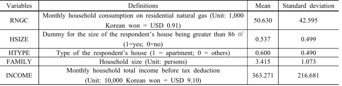
This study covers individual RNGC, using the data collected from a survey of households in Korea. A professional polling firm drew a random sample, reflecting with reasonable accuracy the characteristics of the population. The definitions and sample statistics of variables in the model are reported in Table 1. The sample consists of 2,500 households, with 422 individuals (16.88%) reporting non-consumption of residential NG.
As discussed above, a zero response could be consistent with economic behavior, indicating that the individual derived no benefits from the good or faced income constraints. The mixture model, therefore, appears to be ideally suited for approximating RNGC distribution in our sample, since a fraction of the population has a zero consumption.
3.2 Empirical results
The mixture model is estimated by the maximum likelihood estimation method. Table 2 describes the estimation results. All the estimated parameters in
the model without covariates are statistically significant at the 1 % level. In particular, the estimator for of the mixture model is estimated as
0.1688, which is exactly equal to the observed fraction of individuals reporting non-consumption
(16.88%). Thus, one can suppose that the distribution function of RNGC for the Korean
residents is given by the following formula:
exp
for≥
(6)
Table 2 also presents the results of estimating the mixture model with covariates. The third column (Model A) illustrates the case in which the regressors are only introduced directly into the pdf.
The estimate of parameter equals the proportion of households reporting non-consumption of residential NG. In the fourth column (Model B), the covariates are incorporated into the parameter .
Note that a positive coefficient estimate indicates that households with higher values of the variable are more likely to belong to the non-consumption group of agents, but a negative coefficient estimates implies that households with higher values of the variable are more likely to belong to the positive consumption group.
Thus, the signs of the deep parameters () are as expected. For example, the households whose house size is grater than 86 are less likely to belong to non-consumption group. The households that live in apartment are more likely to belong to consumption group. The household size is positively correlated with the likelihood of not consuming residential NG. Household income has strongly negative relation to the probability that a household has non-consumption of residential NG. Moreover, all the estimated parameters in the model with covariates are also statistically significant at the 10 Table 1. Definitions and sample statistics of variables in model
Variables Definitions Mean Standard deviation
RNGC Monthly household consumption on residential natural gas (Unit: 1,000
Korean won = USD 0.91) 50.630 42.595
HSIZE Dummy for the size of the respondent’s house being greater than 86
(1=yes; 0=no) 0.537 0.499
HTYPE Type of the respondent’s house (1 = apartment; 0 = others) 0.600 0.490
FAMILY Household size (Unit: persons) 3.415 1.073
INCOME Monthly household total income before tax deduction
(Unit: 10,000 Korean won = USD 9.10) 363.271 216.681
% level. The fifth column (Model C) shows the estimation results of a combination of the two cases where covariates are modeled.
3.3 Goodness-of-fit test
For testing the goodness-of-fit between the observed distribution and the distribution implied by the mixture model estimated here, the Kolmogorov-Smirnov (K-S) procedure proposed by Massey (1951) was used for the mixture model without covariates. Alternatively, test of goodness-of-fit can be used. That test, however, requires grouping the observations into a finite number of intervals in an arbitrary manner. The K-S test does not require such grouping.
The K-S test is based on the maximum difference between the observed and implied distributions. Thus,
max (7) where and are the respective value of the observed and implied cdfs for RNGC, . If the value of does not exceed the critical value at a particular significance level, one cannot reject the null hypothesis that there is no difference between the observed and implied values, and can conclude that the mixture model is well fitted to the data.
The critical values of at the 1% and 5%
levels can be estimated as and
, respectively, where is the Table 2. Estimation results for the mixture model
Parametersa Model without covariates
Model with covariates
Model A Model B Model C
1.6310
(61.89)***
1.7291 (61.17)***
1.6310 (61.89)***
1.7291 (61.17)***
: 68.1780
(70.48)***
68.178 (70.48)***
Constant 38.2746
(13.69)***
38.2746 (13.69)***
HSIZE 14.4780
(8.03)***
14.4780 (8.03)***
HTYPE -7.3224
(-4.10)***
-7.3224 (-4.10)***
FAMILY 5.1848
(6.10)***
5.1848 (6.10)***
INCOME 0.0240
(3.86)***
0.0240 (3.86)***
: 0.1688
(22.53)***
0.1688 (22.53)***
Constant -0.3473
(-1.87)*
-0.3473 (-1.87)*
HSIZE -0.3599
(-2.94)***
-0.3599 (-2.94)***
HTYPE -1.6741
(-13.62)***
-1.6741 (-13.62)***
FAMILY 0.1414
(2.53)**
0.1414 (2.53)**
INCOME -0.0023
(-4.92)***
-0.0023 (-4.92)***
Number of
observations 2,500 2,500 2,500 2,500
Log-likelihood -11,407.36 -11,302.36 -11,262.53 -11,157.52
number of data points. The value of is equal to 96. The value of given by equation (7) is computed as 0.0830 and is less than the critical values, and .
Therefore, the K-S goodness-of-fit test does not reject the hypothesis that the RNGC distribution is approximated by the mixture model given in equation (6) at both the 1 and 5% significance levels. We may conclude that the mixture model gives a good fit to the observed monthly RNGC data.
4. Conclusion
Approximating RNGC distribution from individual survey data is complicated by zero responses in the sample. The author proposed and applied the mixture model, where the distribution was allowed to have a possible point mass at zero.
The probability of zero RNGC, represented by parameter , was separately identified and could be consistently estimated. The mixture model could easily capture the common bimodality feature of the RNGC distribution. In addition, when covariates were added to the model, it was found that the probability that an individual has non-consumption of residential natural gas significantly varied with some variables such as household income. The goodness-of-fit test suggests that the data are well represented by the mixture model. As it is computationally easy to estimate, the mixture model offers a practically promising way of approximating the distribution of RNGC data with zero observations.
References
1. Balestra, P., Nerlove, M. "Pooling cross section and time series data in the estimation of a dynamic model: the demand for natural gas." Econometrica, vol. 34, 585-612, (1996) 2. Berndt, E.R., Watkins, G.C. "Demand for
natural gas: residential and commercial markets in Ontario and British Columbia."
The Canadian Journal of Economics, vol..10, 97-111, (1977)
3. Blattenberger, G.R, Taylor, L.D., Rennhack, R.D. Natural gas availability and the residential demand for energy. The Energy Journal, vol. 4, 23-45, (1983)
4. Bloch, F.E. Residential demand for natural gas. Journal of Urban Economics, vol. 7, 371-383, (1980)
5. BP. Statistical review of world energy.
Available from: http://www.bp.com (2012) 6. Dursun, B., Alboyaci, B. An evaluation of
wind energy characteristics for four different locations in Balikesir. Energy Sources, Part A:
Recovery, Utilization, and Environmental Effects, vol. 33, 1086-1103, (2011)
7. Emami, N., Behbahani-Nia, A. The statistical evaluation of wind speed and power density in the Firouzkouh region in Iran. Energy Sources, Part A: Recovery, Utilization, and Environmental Effects, vol. 34, 1076-1083, (2012)
8. Lim, H.-J., Yoo, S.-H. Natural gas consumption and economic growth in Korea:
a causality analysis. Energy Sources Part B:
Economics, Policy, and Planning, vol. 7, 169-176, (2012)
9. Massey, F.J. The Komogorov-Smirnov test for goodness for fit. Journal of American Statistical Association, vol. 46, 68-78, (1951) 10. McLachlan, G.J., Basford, K.E. Mixture
models. New York: Marcel Dekker (1988) 11. Yoo, S.-H. A note on approximation of mobile
communications consumption distribution function using a mixture model. Journal of Applied Statistics, vol. 31, 747-752, (2004) 12. Yoo, S.-H., Lim, H.-J, Kwak, S.-J.
Estimating the residential demand function for natural gas in Seoul with correction for sample selection bias. Applied Energy, vol.
86, 460-465, (2009)