고성능 LDPC 코드를 생성하기 위한 최적화된 알고리듬
서희종*
An Optimized Algorithm for Constructing LDPC Code with Good Performance
Hee-Jong Suh
*요 약
본 논문에서, 성능 좋은 LDPC(Low density parity check) 코드을 위한 태너(Tanner) 그래프를 생성하는 알 고리듬을 제안한다. 이 알고리듬은 뎁스 컨스트렌트(depth constraints)를 유지하면서 태너 그래프의 새로운 가 지를 생성한다. 이 알고리듬은 그래프의 스토핑 셑(stopping set)을 효과적으로 줄이고, 기존의 다른 알고리듬 보다도 낮은 계산복잡도를 갖는다. 모의시험을 통해서 이 알고리듬의 개선된 성능을 확인 할 수 있었다.
ABSTRACT
In this paper, an algorithm having new edge growth with depth constraints for constructing Tanner graph of LDPC(Low density parity check) codes is proposed. This algorithm reduces effectively the number of small stoping set in the graph and has lower complexity than other algorithm. The simulation results shows the improved performance of the LDPC codes constructed by this algorithm.
키워드
LDPC, Stopping Set, ACE, PEG LDPC, 스토핑 셑(Stopping Set), ACE, PEG
* 교신저자(corresponding author) : 전남대학교 전자통신공학과([email protected])
접수일자 : 2013. 06. 10 심사(수정)일자 : 2013. 07. 23 게재확정일자 : 2013. 08. 23
Ⅰ. Introduction
The Low density parity check(LDPC) code becomes one of the best codes because of their low-complexity iterative decoding algorithm and capacity approaching performance[1], and the code attracts more and more researchers' attention to do work in recent years. To construct the good LDPC code, the bipartite graph was considered as an important part. The performance of low density
parity check codes could be improved by optimizing the Tanner graph of this code.
A variety of LDPC code with Tanner graph optimization algorithm is appeared from 1999, and these proposed algorithm can reduce the graph of the stopping set, and improve the performance of the code.
To improve the performance, there are algo-
rithms which are using the girth-conditioning
techniques to increase the girth (shortest cycle
length) of LDPC codes. In 2001, D. M. Arnold et al.
put forward the PEG(Progressive Edge Growth) algorithm[2], this algorithm is through the heuristic search method, and constructing Tanner graphs with large girth by establishing edges or connections progressively between symbols and check nodes in an edge-by-edge manner.
And in 2004, there was the ACE(Approximate Cycle Extrinsic message degree) algorithm by T.
Tian et al. to improve the connectivity of the Tanner graph.[3], this algorithm is different from the previous methods by emphasizing the connectivity as well as the length of cycles. There appeared several improved ACE algorithms [4,5].
But the PEG algorithm is a greedy algorithm, to enlarge the girth, and not to consider about the connectivity of the graph. The ACE algorithm is too complicated, in this algorithm, a list is randomly generated, test cycles and calculate each new cycle with ACE value to determine whether it accord with ACE standard or not. In case of discordance, the list must be generated again.
In this paper, based on ACE and PEG algorithm, a new improved algorithm having edge growth with depth constraints for constructing Tanner graph of LDPC codes is proposed. In this algorithm there is the number of stoping set effectively reduced in the graph and this algorithm has lower complexity than ACE algorithm. With simulation we could see that the performance of LDPC codes which constructed with the new algorithm is better than other’s one.
In Section Ⅱ, definitions related with LDPC are explained. In Section Ⅲ an algorithm having new edge growth with depth constraints for constructing Tanner graph of LDPC codes is proposed. In Section Ⅳ, there are the result of experiments for comparison of the proposed algorithm with PEG and ACE algorithm. Chapter Ⅴ is conclusions. Next is references.
Ⅱ. LDPC Code
The parity check matrix and its bipartite graph of a LDPC code are as shown Fig. 1. The column and row in the parity check matrix correspond to the variable and check node in the bipartite graph.
There exists an edge between variable and check node if and only if
, where
denotes the element of parity check matrix in the th row and
th column.
Fig 1. Parity check matrix and its bipartite graph LDPC code has a stopping sets[6]. A subset of variable nodes is said to form a stopping set if all its neighboring check nodes are connected to at least twice. In Fig. 1, a stopping set is the subset of variable nodes
. But, if a subset has two neighboring check nodes, the subset is not a stopping set. For an example, a subset
,
,
is not stopping set. since the subset has two neighboring check nodes,
and ,
which are connected to only once. In parity check matrix, the stopping sets also can be determined by the ordinary(not mod 2) sum of the columns. In sum of some columns of the matrix, when 1 does not appear, a vertex set representing the columns are stopping set. The sum of columns is
and there is no 1 in it.
It is proved that a small stopping set means
small minimum distance[7]. To avoid small stopping
sets, we have to make the subset of variable nodes
have many extrinsic edges. The quantities of these
extrinsic edges defines an extrinsic message degree
(EMD).
The EMD of a variable node set is the number of extrinsic constraint nodes of this variable node set[7]. An extrinsic check node of a variable node set is a check node that is singly connected to this set. The EMD of a variable node set is the number of extrinsic check nodes of this variable node set.
The EMD of a stopping set is zero and the number of 1 in the sum of the columns over subset of variable nodes is equal to EMD. In the above example, the sum of column over is
, so the EMD of is 2.
The approximate cycle extrinsic message degree (ACE) is defined[8]. The ACE of a length cycle is ∑
, where
is the degree of the th variable node in this cycle.
When variable nodes and their neighboring check nodes compose of a single cycle, the EMD of these variable nodes is equal to the ACE. However, when they compose of multi-cycles, the ACE becomes an upper bound of EMD. In Fig. 1, variable nodes
,
,
and their neighboring check nodes compose of 6-cycle and ACE is one. However, EMD of these variable nodes is zero since this 6-cycle contains a 4-cycle.
Ⅲ. Algorithm
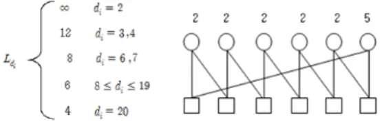
A proposed algorithm uses cycles girth instead of ACE standard in the ACE algorithm. The algorithm is adjusting the parameters of the ACE algorithm. It needs consider cycle girth to add each edge, but not aims to the largest cycles like PEG algorithm. This algorithm uses each variable node degree assigned a target minimum cycle
, parameter standard. For each variable node, when it connects line, the cycles with all bigger degrees than the
, must be generated.
So, this algorithm uses the advantages of the
ACE algorithm and PEG algorithm. The parameter standard
shows as Fig. 2.
Fig 2. Parameter standard limiting cycles The above standard is equivalent to the (6, 2), or (4, 5) standard of the ACE. In the limiting cycles the cycle that length is 12 can only appear when the variables nodes are connected, and the degree is 5. That appearance in the worst case, the rest of the node in the cycle degree is 2, at this time the ACE value of this cycle is 3, also greater than 2, through thus method, it can conform to the 6, 2 standard. Likewise, the cycle that length is 8 can only appear when the variables nodes the degree is 8, so when in the worst case, all the cycle which the length is 8, the ACE value is 6, also satisfies (4, 5) standard.
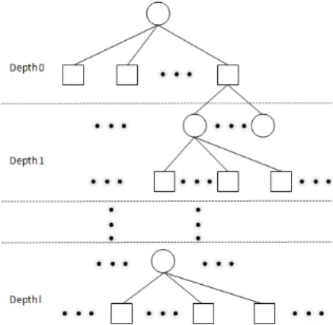
From the PEG algorithm process, progressively establishing edges is drawn between symbol and check nodes in an edge-by-edge manner, as show in Fig. 3. The shortest cycle passing through edge-by-edge is guaranteed to be no shorter than
. The degree of variable nodes corresponding to the minimum depth standard is used instead of cycle length standard.
is as the check nodes set that the length to less than . It means that the graph is from the point of
, including the set of check nodes with depth .
is the rest of the nodes check nodes set
, removing the
. When edge is added, if choosing from the set
, it will appear a cycle that the length is less than , but if choosing from the set
, it will not appear a cycle that the
length is less than . So a node is chosen from the set
. Different from the PEG algorithm, the degree
of each variable node a minimum depth number
are given. If the variable node has degree
, when it extended to the depth
, it will not extended any more, and choose a node from the set
, This limits the length of the cycle which must be greater than
. Then it can limit the length of the cycle.
Fig. 3 Tree constructing the shortest cycles of the algorithm(Variable nodes indicated by cycle, check
nodes indicated by block)
At this time, the further transformation of the above standards is needed, and the length of the cycles standard to the depth layer standard must be changed. Corresponding depth layer standard is given in Table 1.
Table 1. The variable node degree and minimum depth standard
The number of minimum depth
The degree of the variable node
∞
5
3
2 ≤ ≤
1 ≥
Ⅳ. Experiment and Results
With the proposed algorithm which is new algorithm with high performance, the simulations on the its encoding and decoding were done together with the Random, PEG, and ACE algorithm. Code was (1008,504)LDPC code. and the degree distributions of the variable node and check node,
and [8], are as follows.
and
where is LDPC code. And the simulations was under both Erasure channel and Gauss channel.
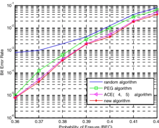
The performance of LDPC code constructed by the proposed algorithm are indicated in Fig. 4, in this Fig. 4, the performance of PEG algorithm, ACE algorithm and proposed algorithm are much better than use a random graph of LDPC code, especially in low delete probability(BEC). The decoding performance with proposed algorithm have similar performance with ACE algorithm and PEG algorithm(we can see in the Fig. 4 when the probability of Erasure is 0.36). But in a high delete probability, such as the probability of Erasure is 0.42, the decoding performance of this proposed algorithm is more outstanding. The outstanding performance can be seen also under the Gauss channel in the Fig. 5. with a low signal-to-noise ratio (BIAWGN) in the channel(from the Fig. 5 when the SNR from 1 to 2). It was verified that the proposed algorithm has better than other algorithms in performance, because of small cycles in iterative decoding. Graph of the code constructed by the proposed algorithm had good connectivity.
After the SNR is 2, the influence of small cycle on
decoding performance is reduced. and the
performance is not outstanding.
0.36 0.37 0.38 0.39 0.4 0.41 0.42 10-6
10-5 10-4 10-3 10-2 10-1
Probability of Erasure (BEC)
Bit Error Rate
random algorithm PEG algorithm ACE( 4, 5) algorithm new algorithm
Fig. 4 Performance comparison of iterative decoding of LDPC codes under the erasure channel
1 1.2 1.4 1.6 1.8 2 2.2
10-4 10-3 10-2 10-1
SNR(dB) BIAWGN
Bit Error Rate
random algorithm PEG algorithm ACE(4,5) algorithm new algorithm
Fig. 5 Performance comparison of iterative decoding of LDPC codes under the gauss channel
Ⅴ. Conclusions
An algorithm having new edge growth with depth constraints for constructing an good Tanner graph of LDPC(Low density parity check) codes is proposed. In this algorithm, the stopping set is reduced in the Tanner graph, and the connectivity of the Tanner graph is increased. Time complexity of this algorithm is ( is the number of node and is the degree). The Time complexity is same with PEG algorithm, and lower than ACE algorithm. But the performance is more outstanding than PEG algorithm(in the Fig. 4 and Fig. 5), The
simulation result shows that the improved performance of LDPC codes constructed by this new algorithm.
References
[1] Robert G. Gallager, "Low-density parity-check codes," MIT Press, Cambridge, Mass., 1963.
[2] D. M. Arnold, E. Eleftheriou, and X. Y. Hu,
"Progressive edge-growth Tanner graphs," in Proc. IEEE Global Telecommunications Conf., Vol. 2, San Antonio, TX, pp. 995-1001, 2001.
[3] T. Tian, C. Jones, J. D. Villasenor, and R. D.
Wesel, "Selective avoidance of cycles in Irregular LDPC code Construction," IEEE Trans. Comm., Vol. 52, pp. 1242-1247, 2004.
[4] Hua Xiao, Amir H. Banihashemi, "Improved Progressive-Edge-Growth(PEG) Construction of Irregular LDPC Codes," IEEE Communications Letters, Vol. 8, 2004.
[5] Sung-Hua Kim, Joon-Sung Kim, Dae-Son Kim,
"LDPC code Construction with Low Error Floor Based on the IPEG Algorithm," IEEE, Communications Letters, Vol. 11, 2007.
[6] C. Di, D. Proietti, "Finite length analysis of low density parity check codes on the binary erasure channel," IEEE Trans. Inf. Theory, Vol.
48, No. 6, pp. 1570-1579, 2002.
[7] T. Tian, C. R. Jones, "Construction of irregular LDPC codes with low error floors," in Proc.
IEEE Int. Conf. Comm, Vol. 5, pp. 3125-3129, 2003.
[8] T, Richardson, A. Shokrollahi, R. Urbanke,
"Design of capacity approaching irregular low density parity check codes," IEEE Trans, Information Theory, Vol. 47, pp. 619-637, 2001.
[9] Hao Chen, H. Suh "An improved Bell- man-Ford algorithm based on SPFA", The Journal of The Korea Institute of Electronic Communication Sciences, Vol. 7, No. 4, pp.
721-726, 2012.
[10] Yanji Liu, H. Suh " A Comparison of Raptor Code Using LDGM and LDPC code", The Journal of The Korea Institute of Electronic Communication Sciences, Vol. 8, No. 1, pp.
65-70, 2013.
[11] Binbin Hu, H. Suh, "Node monitoring algorithm with piecewise linear function approximation for efficient LDPC decoding", The Journal of The Korea Institute of Electronic Communication Sciences, Vol. 6, No. 1, pp. 20-26, 2011.
저자 소개
서희종(Hee-Jong Suh)
![Fig 1. Parity check matrix and its bipartite graph LDPC code has a stopping sets[6]](https://thumb-ap.123doks.com/thumbv2/123dokinfo/5418272.425301/2.774.409.697.351.487/fig-parity-check-matrix-bipartite-graph-ldpc-stopping.webp)