Statistical estimation of crop yields for the Midwestern United States using satellite images, climate datasets, and soil property maps

Statistical estimation of crop yields for the Midwestern United States using satellite images, climate datasets,

and soil property maps

Nari Kim*, Jaeil Cho**, Sungwook Hong***, Kyung-Ja Ha****, Ryosuke Shibasaki***** and Yang-Won Lee*

*Department of Spatial Information Engineering, Pukyong National University

**Division of Plant Biotechnology, Chonnam National University

***Department of Environment, Energy, and Geoinfomatics, Sejong University

****Department of Atmospheric Sciences, Pusan National University

*****Center for Spatial Information Science, The University of Tokyo

Abstract : In this paper, we described the statistical modeling of crop yields using satellite images, climatic datasets, soil property maps, and fertilizer data for the Midwestern United States during 2001-2012. Satellite images were obtained from the Moderate Resolution Imaging Spectroradiometer (MODIS), and climatic datasets were provided by the Parameter-elevation Regressions on Independent Slopes Model (PRISM) Climate Group. Soil property maps were derived from the Harmonized World Soil Database (HWSD). Our multivariate regression models produced quite good prediction accuracies, with differences of approximately 8-15% from the governmental statistics of corn and soybean yields. The unfavorable conditions of climate and vegetation in 2012 could have resulted in a decrease in yields according to the regression models, but the actual yields were greater than predicted. It can be interpreted that factors other than climate, vegetation, soil, and fertilizer may be involved in the negative biases. Also, we found that soybean yield was more affected by minimum temperature conditions while corn yield was more associated with photosynthetic activities. These two crops can have different potential impacts regarding climate change, and it is important to quantify the degree of the crop sensitivities to climatic variations to help adaptation by humans. Considering the yield decreases during the drought event, we can assume that climatic effect may be stronger than human adaptive capacity.

Thus, further studies are demanded particularly by enhancing the data regarding human activities such as tillage, fertilization, irrigation, and comprehensive agricultural technologies.

Key Words : crop yield, satellite image, climate data, soil property, statistical model

Received May 29, 2016; Revised June 3, 2016; Accepted July 7, 2016.

†

Corresponding Author: Yang-Won Lee ([email protected])

This is an Open-Access article distributed under the terms of the Creative Commons Attribution Non-Commercial License (http://creativecommons. org/licenses/by-nc/3.0) which permits unrestricted non-commercial use, distribution, and reproduction in any medium, provided the original work is properly cited

Article

1. Introduction

Information regarding crop yields directly influences domestic and international economies, and can be used as an important data source for determining national food security policies (Hayes and Decker, 1996). Corn and soybeans are the two main grain crops, and their yields in the United States (US) account for 41 and 28% of the total global production, respectively (Taylor and Koo, 2011). The international grain market is becoming unstable due to global climate change, and the prices of corn and soybeans have increased rapidly because of the severe and extensive US drought in 2012. Furthermore, food crisis will get worse in the future because the global demand for grain crops may double around 2050 due to world population growth (Tilman et al., 2011).

Thus, continuous and long-term monitoring of crop yields is required in the world’s major grain producing countries.

Satellite remote sensing techniques are used to continuously observe large areas by analyzing various images. The agricultural applications of satellite remote sensing have enabled its use to estimate the growth and production of grain crops, with many studies producing meaningful achievements (Prasad et al., 2006; Atzberger, 2013). In particular, several studies have focused on the estimation of crop yields through statistical analyses of vegetation indices derived from optical satellite sensors. Allen (1990) estimated the area of crop cultivation and crop yields using satellite images in Iowa. Labus et al. (2002) identified a strong correlation between wheat yields and the Normalized Difference Vegetation Index (NDVI) produced by the Advanced Very High Resolution Radiometer (AVHRR) during the entire growing season in Montana. Ferencz et al. (2004) developed the General Yield Unified Reference Index (GYURI) using satellite images to estimate crop

yields. Moreover, Doraiswamy et al. (2005) assimilated the Leaf Area Index (LAI) obtained from the Moderate Resolution Imaging Spectroradiometer (MODIS) into a numerical crop model to make predictions of corn and soybean yields for Illinois.

Crop yields are influenced by many environmental factors and farming activities. Thus, in addition to satellite images, variables such as climatic elements, hydrological conditions, soil properties, and fertilizer applications have also been used in yield estimations.

Nguu (1987) evaluated the effects of fertilizer inputs of nitrogen and phosphorus on corn yield in Cameroon. Garcia-Paredes et al. (2000) predicted corn and soybean yields by multivariate regression using the physical and chemical properties of soil in Illinois. Prasad et al. (2006) conducted multivariate regressions for corn and soybean yields using MODIS NDVI, precipitation, surface temperature, and soil moisture in Iowa. Ren et al. (2008) also undertook a regression analysis for the yield of winter wheat using MODIS NDVI and weather station data in Shandong, China. Kim et al. (2014) presented a statistical estimation of corn and soybean yields using MODIS products and climatic variables for the US Midwest.

Previous statistical approaches have been successful in estimating crop yields, using various datasets. However, some of them could not comprehensively assess the factors affecting crop yields simply by focusing on the partial relationships between crop yields and individual variables. Not all of them could sufficiently investigate spatiotemporal patterns of crop productivity or the cause-and-effect relationships underlying the crop yields and various framing and environmental factors. Extreme climate events such as drought should be taken into account when examining the characteristics of the yield changes of grain crops. It is also necessary to analyze crop yields using a longer time-series dataset for large areas to improve the accuracy of predictions.

This paper describes the statistical modeling of corn

and soybean yields using a combination of vegetation, climate, soil, and farming factors in the Midwestern US for the period of 2001-2012 and discusses the spatial and temporal characteristics of crop yields according to comprehensive environmental factors, particularly under conditions of drought. The fourteen variables used in multivariate regression models included different types of vegetation indices; climate variables, such as precipitation and temperature;

physical and chemical properties of soil, such as bulk density, acidity, sodicity, and salinity; and fertilizer inputs, to estimate the yearly yields of corn and soybeans. Our multivariate regression models were trained using a ten year dataset for the period of 2001- 2010 and were validated by comparing the predictions of 2011 and 2012 to the yield statistics provided by the National Agricultural Statistics Service (NASS) of the United States Department of Agriculture (USDA).

2. Data and Method

1) Data Processing

The US is one of the world’s largest grain exporters, and the Midwestern US is a major

agricultural region where various crops are cultivated over broad areas, with corn and soybeans being dominant. In general, corn and soybeans are planted in mid-May, mature in September, and are harvested by late October (Xin et al., 2013). Hence, we used data for the period between May and October as the growing season for corn and soybeans. Our study area (Fig. 1) included 305 counties in the four states (99 in Iowa, 87 in Minnesota, 53 in North Dakota, and 66 in South Dakota), which were selected because the area of cropland exceeded 50% of the county area. For masking the croplands, we extracted the pixels that were recorded as cropland (land-cover ID = 12) throughout the twelve years (2001-2012) from the MODIS land-cover product. For the estimation of corn and soybean yields in the study area, we constructed a database for the period of 2001-2012 including satellite images, climate variables, soil property maps, fertilizer inputs, and yield statistics, as shown in Table 1.

Satellite images acquired from Terra MODIS includes the vegetation indices with 1-km spatial resolution, such as NDVI, LAI, and the Enhanced Vegetation Index (EVI). NDVI is the most widely used vegetation index indicating the vitality of vegetation, chlorophyll content, or photosynthetic

Fig. 1. (a) Pixels recorded as cropland (land-cover ID = 12 in the MODIS product) throughout the twelve years (2001-2012);

(b) Counties in which the area of cropland exceeded 50% of the total area.

(a) (b)

activity. EVI responds more sensitively to highly vegetated locations than NDVI (Townshend et al., 1991; Huete et al., 2002). LAI denotes the ratio of leaf area per unit area and is conventionally used as a proxy of biomass of leaves (Sellers, 1985) that can be calculated using the Fraction of Photosynthetically Active Radiation absorbed by vegetation (FPAR).

Climate factors include the 4-km monthly maximum, minimum, and mean air temperatures (Tmax, Tmin, and Tmean) and PreciPiTation (PPT) provided by the Parameter-elevation Regressions on Independent Slopes Model (PRISM) Climate Group (Daly et al., 1994; Daly et al., 2008). Tmax and Tim are the monthly averages of the daily maximum temperatures and the daily minimum temperatures, respectively.

Also, Tmean is the monthly average of the daily mean temperatures. The 8-day or monthly satellite images and climate dataset between May and October were averaged into yearly data for use in the estimation of yearly yields by multivariate regressions.

The physical and chemical properties of soil were extracted from the Harmonized World Soil Database

(HWSD) in a 1-km grid, which was developed by the International Institute for Applied Systems Analysis (IIASA) and the Food and Agriculture Organization (FAO) of the United Nations (UN). We used several properties of the topsoil (0-30 cm) and subsoil (30- 100 cm) layers that can affect crop yields (De la Rosa et al., 1981; Garcia-Paredes et al., 2000; Dam et al., 2005), such as the fraction of clay (T_CLAY and S_CLAY), bulk density (T_BD and S_BD), pH (T_pH and S_pH), calcium carbonate (T_CaCO3 and S_CaCO3), exchangeable sodium percentage (T_ESP and S_ESP), and electrical conductivity (T_ECE and S_ECE) - prefix “T” and “S” were attached for topsoil and subsoil properties, respectively. BD represents the compaction of soil by the ratio of the mass of oven- dried soil to its bulk volume. pH is a measure of the acidity or alkalinity of soil, and CaCO3 is the percentage calcium carbonate (lime) content in the soil. ESP indicates the degree of saturation of the soil exchange complex with sodium, which is calculated as the proportion of sodium among the exchangeable cations in soil. ECE is a measure of the salt Table 1. Summary of the dataset used in multivariate regression models in this study

Data Spatial Resolution Temporal Resolution Source

Vegetation

NDVI

1 km Monthly NASA

EOSDIS

EVI

LAI 8-day

Climate

Precipitation (PPT)

4 km Monthly PRISM

Climate Group Minimum air temperature (Tmin)

Maximum air temperature (Tmax) Mean air temperature (Tmean)

Soil Harmonized World Soil Database* 1 km - IIASA

Fertilizer Nitrogen County Yearly USGS

Yield Soybeans Corn County Yearly USDA

* See Table 2 for more detail of soil properties.

1) EOSDIS (The Earth Observing System Data and Information System) (http://reverb.echo.nasa.gov/reverb/) 2) PRISM (The Parameter-elevation Regressions on Independent Slopes Model) (http://www.prism.oregonstates.edu/) 3) IIASA (The International Institute for Applied Systems Analysis) (http://webarchive.iiasa.ac.at/Research/LUC/External-World-

soil-database/HTML/)

4) USGS (U.S. Geological Survey) (https://catalog.data.gov/dataset/county-level-estimates-of-nitrogen-and-phosphorus-from- commercial-fertilizer-for-the-1987-2006)

5) USDA (U.S. Department of Agriculture) (http://quickstats.nass.usda.gov)

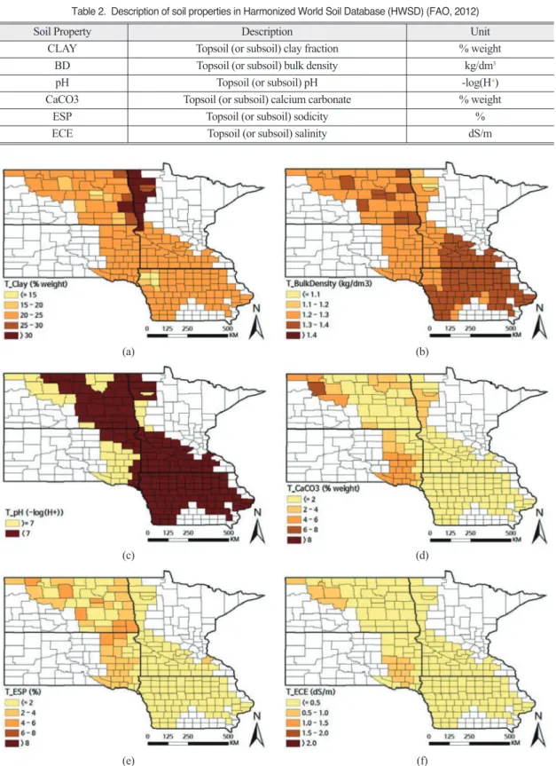
Fig. 2. Spatial distribution of the topsoil and subsoil properties extracted from HWSD: (a) Topsoil clay fraction, (b) Topsoil bulk density, (c) Topsoil pH, (d) Topsoil CaCO3, (e) Topsoil ESP, (f) Topsoil ECE, (g) Subsoil clay fraction, (h) Subsoil bulk density, (i) Subsoil pH, (j) Subsoil CaCO3, (k) Subsoil ESP, Subsoil ECE.

(e)

(a) (b)

(c) (d)

(f)

Table 2. Description of soil properties in Harmonized World Soil Database (HWSD) (FAO, 2012)

Soil Property Description Unit

CLAY Topsoil (or subsoil) clay fraction % weight

BD Topsoil (or subsoil) bulk density kg/dm

pH Topsoil (or subsoil) pH -log(H

)

CaCO3 Topsoil (or subsoil) calcium carbonate % weight

ESP Topsoil (or subsoil) sodicity %

ECE Topsoil (or subsoil) salinity dS/m

concentration in soil at 25°C (FAO, 2012). These variables are summarized in Table 2 and shown as a county-level aggregation in Fig. 2.

Fertilizer information includes the nitrogen input, which is the main fertilizer component responsible for leaf growth (Nguu, 1987). Ruddy et al. (2006) and Gronberg and Spahr (2012) compiled a database of county-level annual inputs of nitrogen using

commercial fertilizer sales data in the US for the period of 1987-2006. Annual changes in nitrogen fertilizer inputs were not significant (Iowa: 1.5%, Minnesota: 0.8%, North Dakota: 5.2%, and South Dakota: 7.1%, respectively) and, therefore, the average of each county during 1987-2006 was used as the value for the period 2007-2012 when no data were available.

Fig. 2. Continued.

(k)

(g) (h)

(i) (j)

(l)

The datasets for vegetation, climate, and soil property were aggregated for each county by using a zonal statistics function, which is a method to summarize pixel values in a given zone. As a reference dataset for building regression models and their validations, county-level yield statistics of corn and soybeans during 2001-2012 were obtained from the Quick Stats (http://quickstats.nass.usda.gov) of the NASS/USDA, which provides reliable crop survey data at the county, state, agricultural district, and national levels.

2) Statistical Modeling

The Ordinary Least Squares (OLS) regression, which is commonly used for crop yield models, was used to minimize the residual sum of squares in the following formula:

y = β

+ β

x

+ β

x

+ … + β

x

+ ε (1) where y represents a response variable, x

to x

are explanatory variables, β

is the intercept, β

to β

indicate the slopes of the relationship between the response variable ( y) and explanatory variables (x

to x

), and ε is the error term.

In this study, the response variables were the yield statistics for corn and soybeans, and the explanatory variables were selected from the fourteen variables for vegetation indices (NDVI, EVI, and LAI), climatic elements (PPT, Tmin, Tmax, and Tmean), topsoil or subsoil properties (CLAY, BD, pH, CaCO3, ESP, and ECE), and nitrogen fertilizer inputs (NTRG). The subsoil properties (S_CLAY, S_BD, S_pH, S_CaCO3, S_ESP, and S_ECE) were included in the variables for the corn model whereas the topsoil properties (T_CLAY, T_BD, T_pH, T_CaCO3, T_ESP, and T_ECE) were used in the soybean model.

This is because the main parts of corn root are generally located below 30 cm and those of soybean root are distributed near the surface (Gao et al., 2010).

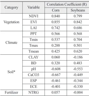
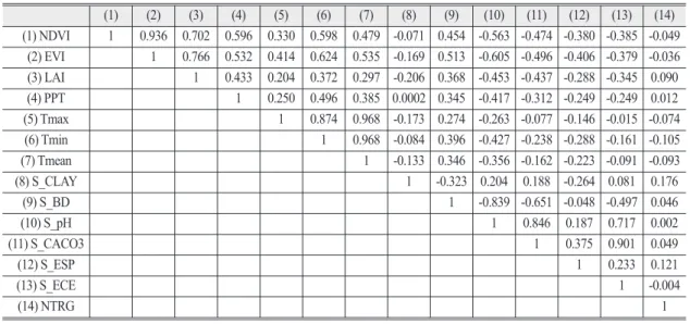
Correlation coefficients (R) were first calculated prior

to selecting appropriate explanatory variables from the fourteen candidates (Table 3) to assess the relationships with the response variables. We then examined the dependencies among the fourteen variables to check the possible duplication or redundancy of the variables (Table 4 and 5). To determine such duplication in a more formalized way, the Variation Inflation Factor (VIF) was calculated as a criterion of the multicollinearity of an explanatory variable with regard to the other explanatory variables. The VIF of the j-th explanatory variable is expressed as:

VIF(x

) = (2) where R

is the R-squared value for the regression of x

against the other covariates (a regression that does not involve the response variable y). The VIF indicates how much x

is correlated with the other explanatory variables. An exploratory variable with a very high VIF can be considered redundant and should be removed from the regression equation.

According to the criterion VIF >10 for existence of 1 _ R 1

Table 3. Correlation coefficients of the variables regarding corn and soybean yields, 2001-2010

Category Variable Correlation Coefficient (R) Corn Soybeans

Vegetation NDVI 0.840 0.799

EVI 0.855 0.842

LAI 0.742 0.686

Climate

PPT 0.566 0.568

Tmin 0.537 0.704

Tmax 0.288 0.501

Tmean 0.425 0.620

Soil*

CLAY 0.060 -0.186

BD 0.320 0.483

pH -0.608 -0.553

CaCO3 -0.667 -0.449

ESP -0.461 -0.344

ECE -0.401 -0.330

Fertilizer NTRG 0.057 -0.004

* Subsoil properties for corn and topsoil properties for

soybeans.

multicollinearity (Kutner et al., 2004), we excluded EVI, Tmax, Tmean, and CaCO3 from the explanatory variables. The ten variables of NDVI, LAI, PPT, Tmin, CLAY, BD, pH, ESP, ECE, and NTRG (Table 6) were then selected for our multivariate regression models.

The response variable and the ten explanatory variables were normalized in the form of a z-score, calculated as Z = (v _ μ)/σ, where v is an individual value, μ is the mean, and σ is the standard deviation for all of the data during 2001-2010. This is because Table 4. Matrix for correlation coefficients of the corn variables, 2001-2010

(1) (2) (3) (4) (5) (6) (7) (8) (9) (10) (11) (12) (13) (14)

(1) NDVI 1 0.936 0.702 0.596 0.330 0.598 0.479 -0.071 0.454 -0.563 -0.474 -0.380 -0.385 -0.049 (2) EVI 1 0.766 0.532 0.414 0.624 0.535 -0.169 0.513 -0.605 -0.496 -0.406 -0.379 -0.036 (3) LAI 1 0.433 0.204 0.372 0.297 -0.206 0.368 -0.453 -0.437 -0.288 -0.345 0.090 (4) PPT 1 0.250 0.496 0.385 0.0002 0.345 -0.417 -0.312 -0.249 -0.249 0.012

(5) Tmax 1 0.874 0.968 -0.173 0.274 -0.263 -0.077 -0.146 -0.015 -0.074

(6) Tmin 1 0.968 -0.084 0.396 -0.427 -0.238 -0.288 -0.161 -0.105

(7) Tmean 1 -0.133 0.346 -0.356 -0.162 -0.223 -0.091 -0.093

(8) S_CLAY 1 -0.323 0.204 0.188 -0.264 0.081 0.176

(9) S_BD 1 -0.839 -0.651 -0.048 -0.497 0.046

(10) S_pH 1 0.846 0.187 0.717 0.002

(11) S_CACO3 1 0.375 0.901 0.049

(12) S_ESP 1 0.233 0.121

(13) S_ECE 1 -0.004

(14) NTRG 1

Table 5. Matrix for correlation coefficients of the soybean variables, 2001-2010

(1) (2) (3) (4) (5) (6) (7) (8) (9) (10) (11) (12) (13) (14)

(1) NDVI 1 0.937 0.699 0.599 0.364 0.614 0.503 -0.072 0.443 -0.552 -0.444 -0.364 -0.338 -0.056 (2) EVI 1 0.767 0.533 0.442 0.636 0.555 -0.172 0.505 -0.593 -0.474 -0.390 -0.345 -0.041 (3) LAI 1 0.431 0.229 0.381 0.314 -0.209 0.365 -0.440 -0.419 -0.279 -0.321 0.088 (4) PPT 1 0.261 0.496 0.389 0.005 0.332 -0.411 -0.299 -0.246 -0.230 0.013

(5) Tmax 1 0.883 0.971 -0.181 0.292 -0.274 -0.083 -0.141 -0.009 -0.084

(6) Tmin 1 0.970 -0.091 0.396 -0.422 -0.224 -0.274 -0.132 -0.111

(7) Tmean 1 -0.141 0.354 -0.358 -0.158 -0.214 -0.072 -0.100

(8) T_CLAY 1 -0.346 0.212 0.201 -0.276 0.094 0.179

(9) T_BD 1 -0.828 -0.646 -0.020 -0.494 0.042

(10) T_pH 1 0.843 0.164 0.713 0.009

(11) T_CACO3 1 0.356 0.898 0.052

(12) T_ESP 1 0.214 0.113

(13) T_ECE 1 -0.011

(14) NTRG 1

Table 6. Variation inflation factor (VIF) of selected explanatory variables for corn and soybean yields, 2001-2010 Variable Variation inflation factor (VIF)

Corn Soybeans

NDVI 3.343 3.357

LAI 2.183 2.264

PPT 1.670 1.667

Tmin 1.978 1.880

CLAY 1.151 1.487

BD 2.062 3.869

pH 3.289 6.141

ESP 1.450 1.428

ECE 3.536 2.391

NTRG 1.072 1.177

normalized values allow for comparisons among the regression coefficients even though they originally had different units. pH was the only exception in the normalization. An appropriate soil pH for corn and soybeans is generally 6.0-7.0 (Bongiovanni et al., 2000; Espinoza et al., 2004), and the T_pH values in the study area ranged between 6.132 and 7.437 while S_pH values were between 5.674 and 8.085. Thus, we divided the study area into two groups of weak acid (pH <7.0) and alkaline (pH ≥7.0) conditions (Fig.

2(c) and 2(i)), which were denoted as a binary variable in the regression equation (S_pH_Bin for corn and T_pH_Bin for soybean, respectively). Finally, the multivariate regression models for corn and soybean yields were expressed as follows:

Yield

= β

+ β

X

+ β

X

+ β

X

+ β

X

+ β

X

+ β

X

(3) + β

X

+ β

X

+ β

X

+ β

X

Yield

= β

+ β

X

+ β

X

+ β

X

+ β

X

+ β

X

+ β

X

+ β

X

+ β

X

(4) + β

X

+ β

X

3. Results and Discussion

1) Evaluation of Regression Models

The R-squared (R

) values for the corn and soybean models were 0.792 and 0.771, respectively, which indicates the strong explanatory power of the models.

Due to the normalization of the response and

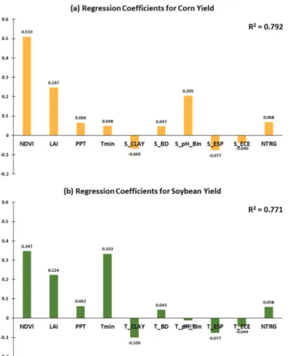
Fig. 3. Regression coefficients derived from normalized response and explanatory variables; (a) corn, (b) soybeans (p-value < 0.05

except for T_pH_Bin in the soybean model).

explanatory variables, we could directly compare the regression coefficients in terms of the degree of impact on the corn and soybean yields (Fig. 3). The characteristics of β

and β

were remarkable.

β

had the greatest coefficient for both corn (0.510) and soybeans (0.347). It was approximately 10 times greater than β

for corn (0.048), but was almost the same as β

for soybeans (0.333). When comparing the β

of corn and soybeans, we found the impact of Tmin on soybean yields was much greater (approximately seven times) than on corn yields.

For the two vegetation indices, β

were approximately 1.5-2 times greater than β

for corn and soybeans. Although both indices were very closely associated with crop growth (Sellers, 1985;

Islam and Bala, 2008; Bala and Islam, 2008), the coefficients indicates that the corn and soybean yields were more related to the NDVI than to the LAI. It is consistent with the previous remote sensing studies which have used the NDVI as the crop photosynthetic activity. In addition, both β

and β

were higher for corn than for soybeans.

In the case of climate variables, corn yields were somewhat more influenced by PPT than by Tmin. In the Midwestern US where drought is frequent, corn is usually more sensitive to water stress than heat stress due to its tall canopy and broad foliage (Classen and Shaw, 1970; Carlson, 2013). In contrast, the β

of soybeans was approximately five times greater than β

. It indicates the significance of a higher Tmin to ensure soybean productivity, but further investigations will be necessary for the reason. Indeed, soybean is weaker to cold weather. The temperature range for soybean growth is 15-26°C (Liu et al., 2008), while for corn growth the range is 5-35°C (Neild and Newman, 1987). Soybean yields in the areas with T

<15°C were lower than average in the four states, while this was not necessarily the case for corn yields.

In addition, Tmin can significantly affect the flowering time of soybeans than Tmax (Thomas et al.,

1981; Wallace, 1986).

Sandy loam, loam, and silt loam are suitable soil textures for corn and soybeans because they have favorable drainage conditions due to the low proportion of clay components (Espinoza and Ross, 2004; Jégo et al., 2015). The regression results also indicated negative coefficients for both corn and soybeans, and the impact of drainage was greater for soybeans than for corn. However, further studies will be necessary to identify the drainage effect by clay content under consideration of irrigation patterns.

Bulk density as an indicator of soil compaction may affect root growth (Allmaras et al., 1988). A bulk density below 1.4 kg/dm

is appropriate for the growth of corn and soybeans (FAO, 2012), and the soils in all the counties in the study area had a bulk density less than 1.47 kg/dm

(Fig. 2(b) and 2(h)). For this reason, β

and β

might be positive, but the impact of soil bulk density on corn and soybean yields should be reexamined in more detail in terms of root morphology. As in Fig. 2(c), approximately 82% of the topsoil in the study area satisfied the pH condition (i.e., 6.0-7.0) while approximately 54% of the subsoil satisfied the condition, which indicates the β

for corn were higher than the β

for soybeans because the subsoil pH could be more critical (half of the subsoil pH was suitable but the other half was not).

The regression coefficients for sodicity and salinity were negative, because the soil sodicity and salinity can cause vegetation stress, obstructing crop growth and productivity (Maas, 1984; Abrol et al., 1988;

Wiegand et al., 1996; Yamaguchi and Blumwald, 2005; Shabhax and Ashraf, 2013).

The values of β

for both corn and soybeans

were as great as β

, which implies the significance

of nitrogen fertilizer were comparable with

precipitation (Nguu, 1987). The starter nitrogen

application can positively affect soybean yields

(Wood et al., 1993), but excessive inputs of nitrogen

fertilizer can interrupt the nitrogen fixation and may

have negative impacts on soybean yields (Weber, 1966; Beard and Hoover, 1971; Deibert et al., 1979).

In general, fertilization is a limiting factor, not a proportional variable to the crop yields. However, the role of nitrogen input could be enhanced when it was combined with enough precipitation in the study area.

Further investigation may be required to reveal the cause and effect of fertilization and crop yields in more detail.

2) Prediction of Crop Yields

Using the regression equations derived from the period 2001-2010, we made predictions of the corn and soybean yields for 2011 and 2012. These predictions were in the form of the normalized yield values and were converted into the original values using the z-score formula. Table 7 presents the validation results, which were relatively favorable in terms of the error statistics. The mean absolute error (MAE) was 0.726 ton/ha (2011) and 1.046 ton/ha (2012) for corn yields, and 0.252 ton/ha (2011) and 0.392 ton/ha (2012) for soybean yields, respectively.

These values corresponded to the Mean Absolute Percentage Error (MAPE) of approximately 8-15% in terms of the USDA yield statistics of corn and soybeans. The correlation coefficients between the predictions and the statistics were 0.909 and 0.854 for corn, and 0.903 and 0.877 for soybeans, respectively.

In addition, it was notable that the prediction errors were higher in 2012, presumably due to a severe drought in the Midwestern US (USDA, 2012; USDA- ERS, 2012; Mallya et al., 2013). All of the error statistics, i.e., mean bias, MAE, Root Mean Squared

Error (RMSE), MAPE, and correlation coefficients, worsened slightly in 2012 because the drought decreased crop yields, leading to an increase in the differences between the predictions and the statistics.

Consequently, the regression models were considered to be more appropriate for estimating crop yields in normal years rather than in disaster years.

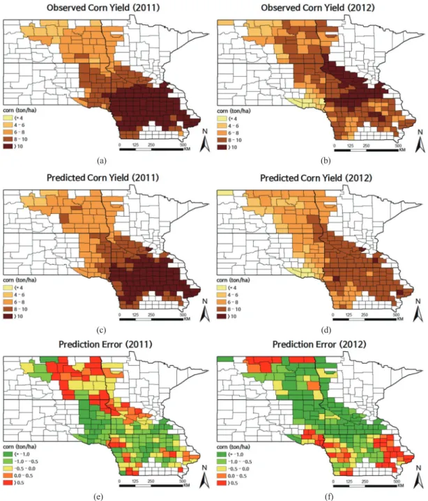
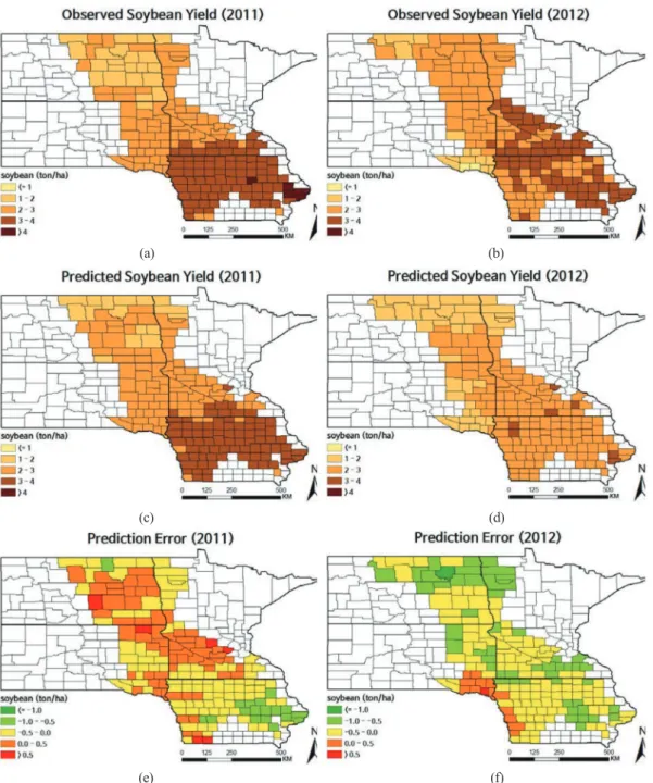
Fig. 4 and 5 represent the yield statistics, predictions, and accuracies for corn and soybeans in 2011 and 2012. Yield patterns were correlated spatially, but the prediction errors did not exhibit significant spatial autocorrelation despite the overall underestimation of the regression models. The underestimation was partly due to the yield growth greater than expected (http://www.nass.usda.gov/

Charts_and_Maps/Field_Crops), so the regression models built from the period of 2001-2010 may not sufficiently reflect the rapid yield increases in 2011 and the abrupt changes of environmental factors in 2012 (Hatfield, 2012). However, the variety of appropriate long-term datasets used in this study meant that, to some extent, our regression models were stable and accurate.

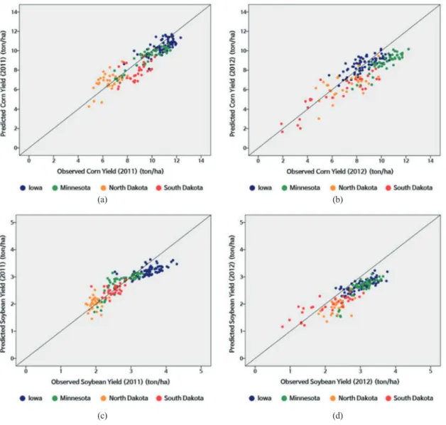
Fig. 6 shows scatter plots of yield predictions against USDA statistics in 2011 and 2012. The colors represent the states each county belongs to: Iowa in navy, Minnesota in green, North Dakota in orange, and South Dakota in red. The accuracy of predictions varied by state, with the MAE of the state with the highest accuracy being approximately half of that for the state with the lowest accuracy. Minnesota had the highest accuracy (MAE = 0.555) and South Dakota had the lowest accuracy (MAE = 1.159) for corn in Table 7. Validation results of the regression models for corn and soybean yields

No. of Counties

(ton/ha) Min Obs.

(ton/ha) Max Obs.

(ton/ha) Mean Obs.

(ton/ha) Mean Bias (ton/ha) MAE

(ton/ha) RMSE (ton/ha) MAPE

(%) R

Corn (2011) 180 4.871 12.334 9.456 -0.350 0.726 0.861 8.144 0.909

Corn (2012) 182 1.883 12.208 8.463 -0.675 1.046 1.240 12.681 0.854

Soybeans (2011) 181 1.715 4.304 2.871 -0.093 0.252 0.313 8.812 0.903

Soybeans (2012) 177 0.780 3.766 2.762 -0.347 0.392 0.442 14.616 0.877

2011 (Fig. 4(e) and 6(a)). For corn in 2012, the accuracy was highest in Iowa (MAE = 0.651) and lowest in Minnesota (MAE = 1.557) as shown in Fig.

4(f) and 6(b). For soybeans, South Dakota had the highest accuracy (MAE = 0.155) and Iowa had the lowest (MAE = 0.342) in 2011 (Fig. 5(e) and 6(c)),

while the accuracies in 2012 were not good overall (Fig. 5(f) and 6(d)). Such variations in accuracy between states may imply the need for local modeling.

The predicted yields were slightly underestimated in accordance with the negative values of the mean bias shown in Table 7. The portions of the negative

Fig. 4. Spatial distributions of corn yield: (a) observed yield in 2011 and (b) in 2012; (c) predicted yield in 2011 and (d) in 2012;

(e) prediction error in 2011 and (f) in 2012.

(e)

(b) (a)

(d) (c)

(f)

biases with regard to actual yields were slightly greater in 2012. The values were approximately -3.7%

(-0.350/9.456) for corn and -3.2% (-0.093/2.871) for soybeans in 2011, but -8.0% (-0.675/8.463) for corn and -12.6% (-0.347/2.762) for soybeans in 2012, which were 2-4 times greater. These abrupt changes

were presumably related to the severe drought in 2012. Conversely, the increase in the negative bias in 2012 was notable, meaning that actual yields were greater than predicted, despite the drought. The unfavorable conditions of climate and vegetation could have resulted in a decrease in yields according

Fig. 5. Spatial distributions of soybean yield: (a) observed yield in 2011 and (b) in 2012; (c) predicted yield in 2011 and (d) in 2012;

(e) prediction error in 2011 and (f) in 2012.

(e)

(b) (a)

(d) (c)

(f)

to the regression models, but the actual yields for corn and soybeans were 8.0 and 12.6% greater than predicted. It can be also interpreted that factors other than climate, vegetation, soil, and fertilizer may be involved in the negative biases, namely the positive actual yields, particularly in 2012. Agricultural technology could be one of the hidden factors (Tambo and Abdoulay, 2012), but further studies are necessary to confirm this.

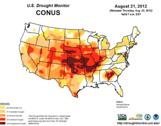
The positive effect in actual yield was considerably larger for soybeans than for corn, partly because the drought endurance of soybeans is stronger than that

of corn (Classen and Shaw, 1970; Sinclair et al., 2007). Fig. 7 shows a map of drought severity in the US in August 2012. The drought was more severe in Iowa and South Dakota than in Minnesota and North Dakota, and it was connected to the decrease in the yield of corn and soybeans in Iowa and South Dakota for the year. In Fig. 6(d), it can be seen that the actual yields of soybeans in Iowa were higher than predicted (i.e., underestimated), while those in South Dakota were lower than predicted (i.e., overestimated), which indicates that crops in Iowa were better able to manage the drought through some adaptation efforts,

Fig. 6. Comparisons between observed and predicted yields for corn ((a) 2011 and (b) 2012) and soybeans ((c) 2011 and (d) 2012).

(c)

(b) (a)

(d)

such as irrigation systems, agricultural technologies, and the development of drought-tolerant crops by Genetically Modified Organism (GMO) or Genetically Engineered Organism (GEO). Thus, a consideration of drought adaption is also necessary for more realistic statistical modelling of crop yields.

4. Conclusions

In this paper, we described the statistical estimation of corn and soybean yields using satellite images, climatic datasets, soil property maps, and fertilizer input data for the Midwestern US during 2001-2012.

We also investigated the unique characteristics of the environmental factors with regard to the yield patterns and discussed the spatial and temporal variations of the yields influenced by the drought, which will be increased due to the climate variability under warmer atmosphere (Wetherald and Manabe, 2002). Our multivariate regression models produced relatively

favorable prediction accuracies, with differences of 8- 15% from the USDA yield statistics of corn and soybeans, although there were some underestimations in the drought year of 2012.

Much scientific effort has been expended to assess the degree of exposure to the negative impact of future climate change, but agricultural sensitivity to the climate change is not well understood although lower crop yields and higher food prices has already been realized under current climate change (IPCC, 2014).

In addition, the studies using process-based crop models are required to reach an acceptable level of confidence by overcoming model-dependency and model-uncertainty (Parry et al., 1999). Therefore, although the crop model approach is scientifically important for understanding the mechanisms of agricultural physiology and ecology, statistical analyses of crop yields using cumulative information about vegetation, climate, soil, and farming activities are necessary for various climate zones and crop types.

Fig. 7. Drought severity map in the US in August 2012 (http://droughtmonitor.unl.edu/).

We found that soybean yield is more affected by minimum temperature conditions while corn yield was more associated with photosynthetic activities.

These two crops can have different potential impacts in relation to climate change, and it is important to quantify the degree of the crop sensitivities to climatic variations to help adaptation by humans. Considering the yield decreases during the drought event, we can assume that climatic effect may be stronger than human adaptive capacity. To identify this issue, further studies are demanded particularly by enhancing the data regarding human activities such as tillage, fertilization, irrigation, and comprehensive agricultural technologies. In addition, the NASS Cropland Data Layer (CDL) for the crop-specific land use maps can be used to distinguish from corn and soybean croplands, which will produce a more reasonable estimation of the crop yields.

Acknowledgment

This work was supported by the Research Grant of Pukyong National University (2014).

References

Abrol, I.P., J.S.P. Yadav, and F.I. Massound, 1988. Salt- affected soils and their management, Food and Agriculture Organization Soils Bulletin. 39.

Allen, J.D., 1990. A look at the remote sensing applications program of the National Agricultural Statistics Service, Journal of official Statistics, 6: 393-409.

Allmaras, R.R., J.M. Kraft, and D.E. Miller, 1988.

Effects of soil compaction and incorporated crop residue on root health, Annual Review of Phytopathology, 26: 219-243.

Atzberger, C., 2013. Advances in remote sensing of

agriculture: Context description, existing operational monitoring systems and major information needs, Remote Sensing, 5: 949- 981.

Bala, S.K. and A.S. Islam, 2008. Estimation of potato yield in and around Munshiganj using remote sensing NDVI data, Institute of Water and Flood Management (IWFM), BUET, Dhaka- 1000, Bangladesh.

Beard, B.H. and R.M. Hoover, 1971. Effect of nitrogen on nodulation and yield of irrigated soybean, Agronomy Journal, 63: 815-816.

Bongiovanni, R. and J. Lowenberg-DeBoer, 2000.

Economics of variable rate lime in Indiana, Precision Agriculture, 2: 55-70.

Carlson, R.E., 2013. Heat stress, plant-available soil moisture, and corn yields in Iowa: a short- and long-term view, Journal of Production Agriculture, 3(3): 293-297.

Classen, M.M. and R.H. Shaw, 1970. Water deficit effects on corn. I. Grain components, Agronomy Journal, 62: 652-655.

Daly, C., R.P. Neilson, and D.L. Philips, 1994. A statistical-topographic model for mapping climatological precipitation over mountainous terrain, Journal of Applied Meteorology, 33(2):

140-158.

Daly, C., M. Halbleib, J.I. Smith, W.P. Gibson, M.K.

Doggett, G.H. Taylor, and J. Curtis, 2008.

Physiographically sensitive mapping of climatological temperature and precipitation across the conterminous United States, International Journal of Climatology, 28:

2031-2064.

Dam, R.F., B.B. Mehdi, M.S.E. Burgess, C.A.

Madramootoo, G.R. Mehuys, and I.R. Callum,

2005. Soil bulk density and crop yield under

eleven consecutive years of corn with different

tillage and residue practices in a sandy loam

soil in central Canada, Soil and Tillage

Research, 84: 41-53.

De la Rosa, D., F. Cardona, and J. Almorza, 1981. Crop yield predictions based on properties of soils in Sevilla, Spain, Geoderma, 25: 267-274.

Doraiswamy, P.C., T.R. Sinclair, S. Hollinger, B.

Akhmedov, A. Stern, and J. Prueger, 2005.

Application of MODIS derived parameters for regional crop yield assessment, Remote Sensing of Environment, 97: 192-202.

Deibert, E.J., M. Bijeriego, and R.A. Olson, 1979.

Utilization of N fertilizer by nodulating and non-nodulating soybean isolines, Agron. J. 71:

717-723.

Espinoza, L. and J. Ross, 2004. Corn production handbook, MP437-2M-2-03N, Little Rock:

University of Arkansas Division of Agriculture Cooperative Extension Service, USA.

FAO/IIASA/ISRIC/ISSCAS/JRC, 2012. Harmonized World Soil Database (version 1.2), FAO, Rome, Italy, and IIASA, Laxenburg, Austria.

Ferencz, C., P. Bognár, J. Lichtenberger, D. Hamar, Gy.

Tarcsai, G. Timár, G, Molnár, Sz., Pásztor, P.

Steinbach, B. Székely, O.E. Ferencz, and I.

Ferencz-Árkos, 2004. I. Crop yield estimation by satellite remote sensing, International Journal of Remote Sensing, 25: 4113-4149.

Gao, Y., A. Duan, X. Qiu, Z. Liu, J. Sun, J. Zhang, and H. Wang, 2010. Distribution of roots and root length density in a maize/soybean strip intercropping system, Agricultural Water Management, 98: 199-212.

Garcia-Paredes, J.D., K.R. Olson, and J.M. Lang, 2000.

Predicting corn and soybean productivity for Illinois soils, Agricultural Systems, 64: 151- 170.

Gronberg, J.M. and N.E. Spahr, 2012. County-level estimates of nitrogen and phosphorus from commercial fertilizer for the conterminous United States, 1987-2006, US Department of the Interior, US Geological Survey.

Hatfield, J., 2012. Agriculture in the Midwest, In: U.S.

National Climate Assessment Midwest Technical Input Report, J. Winkler, J. Andresen, J. Hatfield, D. Bidwell, and D. Brown, coordinators, Available from the Great Lakes Integrated Sciences and Assessments (GLISA) Center.

Hayes, M.J. and W.L. Decker, 1996. Using NOAA AVHRR data to estimate maize production in the United States Corn Belt, International Journal of Remote Sensing, 17: 3189-3200.

Huete, A.R., K. Didan, T. Miura, E.P. Rodriguez, X.

Gao, L.G. Ferreria, 2002. Overview of the radiometric and biophysical performance of the MODIS vegetation indices, Remote Sensing of Environment, 83: 195-213.

IPCC, 2014. Climate change 2014: mitigation of climate change, Contribution of Working Group III to the Fifth Assessment Report of the Intergovernmental Panel on Climate Change, Cambridge University press, Eng.

Islam, A.S. and S.K. Bala, 2008. Assessment of potato phonological characteristics using MODIS- derived NDVI and LAI information, Giscience and Remote Sensing, 45: 454-470.

Jégo, G., E. Pattey, S.M. Mesbah, J. Liu, and I.

Duchesne, 2015. Duchesne, I. Impact of the spatial resolution of climatic data and soil physical properties on regional corn yield predictions using the STICS crop model, International Journal of Applied Earth Observation and Geoinformation, 41: 11-22.

Kim, N., J, Cho, R. Shibasaki, and Y-W. Lee, 2014.

Estimation of corn and soybeans yields of the US Midwest using Satellite imagery and climate dataset, Journal of Climate Research, 9(4): 315-329.

Kutner, M.H., C.J. Nachtsheim, and J. Neter, 2004.

Applied Linear Regression Models (4th ed.),

Mc-Graw-Hill/Irwin. USA.

Labus, M.P., G.A. Nielsen, R.L. Lawrence, R. Engel, and D.S. Long, 2002. Wheat yield estimates using multi-temporal NDVI satellite imagery, International Journal of Remote sensing, 23:

4169-4180.

Liu, X., J. Jin, G. Wang, and S.J. Herber, 2008.

Soybeans yield physiology and development of high-yielding practices in Northeast China, Field Crops Research, 105: 157-171.

Maas, E.V., 1984. Salt tolerance of plants, Handbook of plant science in agriculture, 2: 57-75.

Mallya, G., L. Zhao, X.C. Song, D. Niyogi, and R.S.

Govindaraju, 2013. 2012 Midwest drought in the United States, Journal of Hydrologic Engineering, 18: 737-745.

Neild, R.E. and J.E. Newman, 1987. Growing season characteristics and requirements in the Corn Belt, Cooperative Extension Service, Iowa State University.

Nguu, N.V., 1987. Effect of nitrogen, phosphorus and soil and crop residues management practices on maize (Zea mays L.) yield in ultisol of eastern Cameroon. Fertilizer Research, 14: 135-142.

Parry, M., C. Rosenzweig, A. Iglesias, G. Fischer, and M. Livermore, 1999. Climate change and world food security: A new assessment, Global Environ, Change, 9: 51-67.

Prasad, A.K., L. Chai, R.P. Singh, and M. Kafatos, 2006. Crop yield estimation model for Iowa using remote sensing and surface parameters, International Journal of Applied Earth Observation and Geoinformation, 8: 26-33.

Ren, J., Z. Chen, Q. Zhou, and H. Tang, 2008. Regional yield estimation for winter wheat with MODIS- NDVI data in Shandong, China, International Journal of Applied Earth Observation and Geoinformation, 10: 403-413.

Ruddy, B.C., D.L. Lorenz, and D.K. Mueller, 2006.

County-level estimates of nutrient inputs to the land surface of the Conterminous United

States, 1982-2001, US Department of the Interior, US Geological Survey.

Sellers, P.J., 1985. Canopy reflectance, photosynthesis and transpiration, International Journal of Remote Sensing, 6: 1335-1372.

Shabhaz, M. and M. Ashraf, 2013. Improving salinity tolerance in cereals, Critical Reviews in Plant Sciences, 32: 237-249.

Sinclair, T.R., L.C. Purcel, C.A. King, C.H. Sneller, P.

Chen, and V. Vadez, 2007. Drought tolerance and yield increase of soybean resulting from improve symbiotic N2 fixation, Field Crops Research, 101: 68-71.

Tambo, J.A. and T. Abdoulay, 2012. Climate change and agricultural technology adoption: the case of drought tolerant maize in rural Nigeria, Mitigation and Adaptation Strategies for Global Change, 17: 277-292.

Taylor, R.D. and W.W. Koo, 2011. 2011 Outlook of the U.S. and World corn and soybeans industries, 2010-2020, Agribusiness and Applied Economics Report, 682.

Thomas, J.F., C.D. Raper, and W.W. Weeks, 1981. Day and night temperature effects on nitrogen and soluble carbohydrate allocation during early reproductive growth in soybeans, Agronomy Journal, 73: 577-582.

Tilman, D., C. Balzer, J. Hill, and B.L. Befort, 2011.

Global food demand and the sustainable intensification of agriculture, Proc. of the National Academy of Sciences, 108: 20260- 20264.

Townshend, J.R.G., C.O. Justice, W. Li, C. Gurney, and J. McManus, 1991. Global land cover classification by remote sensing: present capabilities and future capabilities, Remote Sensing of Environment, 35: 243-255.

USDA, 2012. USDA announces streamlined disaster

designation process with lower emergency loan

rates and greater CRP flexibility in disaster

areas, USDA Newsroom.

USDA Economic Research Service (USDA-ERS), 2012. U.S. drought 2012: Farm and food impacts.

Wallace, D.H., 1986. Physiological genetics of plant maturity, adaptation, and yield, in plant breeding review, Volume 3 (ed J. Janick), John Wiley & Sons, Inc., Hoboken, NJ, USA: 94- 99.

Weber, C.R., 1966. Nodulating and nonnodulating isolines: II. Response to applied nitrogen and modified soil conditions, Agronomy Journal, 58: 46-49.

Wetherald, R.T. and S. Manabe, 2002. Simulation of hydrologic changes associated with global warming, Journal of Geophysical Research, 107: 4379-4393.

Wiegand, C., G. Anderson, S. Lingle, and D. Escobar,

1996. Soil salinity effects on crop growth and yield-Illustration of an analysis and mapping methodology for sugarcane, Journal of Plant physiology, 148: 418-424.

Wood, C.W., H.A. Torbert, and D.B. Weaver, 1993.

Nitrogen fertilizer effects on soybean growth, yield, and seed composition, Journal of Production Agriculture, 6: 354-360.

Xin, Q., P. Gong, C. Yu, L. Yu, M. Broich, A.E. Suyker, and R.B. Myneni, 2013. A production efficiency model-based method for satellite estimates of corn and soybean yields in the Midwestern US, Remote Sensing, 5: 5926- 5943.

Yamaguchi, T. and E. Blumwald, 2005. Developing

salt-tolerant crop plants: challenges and

opportunities, Trends Plant Science, 10: 615-

620.