Spatial and Temporal Variability of Phytoplankton at Hwadang-ri, Goseng-gun
Man Ki Kang
1and Man Kyu Huh
2*
1
Department of Data Information Science, College of Natural Sciences & Human Ecology, Dongeui University, Busan 614-714, Korea
2
Department of Molecular Biology, College of Natural Sciences & Human Ecology, Dongeui University, Busan 614-714, Korea
Received March 4, 2014 /Revised May 2, 2014 /Accepted May 7, 2014This study describe seasonal patterns in the variation of phytoplankton frequency in the water surface and basal layers and their spatial distributions at seven stations in Hwadang-ri, Goseng-gun in 2013.
The phytoplankton community at Hwadang-ri was very diverse, with 60 taxa identified, representing three classes. Diatoms (Bacillariophyceae) exhibited the greatest diversity, with 41 taxa identified.
These were followed by the dinoflagellates Dinophyceae, Cryptophyceae, and Eugenophyceae, with 16 taxa, two taxa, and one taxon, respectively. Water surfaces were shown with the relative individual density or abundance across areas. Except in January, Shannon–Weaver indices of diversity of the wa- ter surface layer were lower than those of the basal layer. In addition, evenness indices of the basal layer were higher than those of the water surface layer, except in January. For the community as a whole, the values of ß-diversity were low for the seven stations: 1.125 for the water surface layer and 1.481 for the basal layer. Seasonal values for ß-diversity were similar at the seven stations: 1.725 for the water surface layer and 1.347 for the basal layer. The phytoplankton community showed high taxonomic homogeneity in all four seasons, in addition to similar trends in seasonal development at depths in the same stations. However, the size distribution of the abundance and biomass showed a statistically significant west-east difference.
Key words : Hwadang-ri, phytoplankton, size–frequency distribution, spatial patterns, ß-diversity
*Corresponding author
*Tel : +82-51-890-1521, Fax : +82-51-890-1529
*E-mail : [email protected]
This is an Open-Access article distributed under the terms of the Creative Commons Attribution Non-Commercial License (http://creativecommons.org/licenses/by-nc/3.0) which permits unrestricted non-commercial use, distribution, and reproduction in any medium, provided the original work is properly cited.
Journal of Life Science 2014 Vol. 24. No. 5. 532~542 DOI : http://dx.doi.org/10.5352/JLS.2014.24.5.532
Introduction
Phytoplankton is photosynthesizing microscopic organ- isms and the autotrophic components of the plankton community. They inhabit most the upper sunlit layer of al- most all oceans and bodies of fresh water. Despite their in- finitely small size in comparison to other marine organisms, these tiny creatures occupy an immensely important eco- logical niche. They are agents for very important primary production of earth. By the action of the sun’s rays on chlor- ophyll (light absorbing pigments found within the phyto- plankton cell) these plants produce carbohydrates, proteins, fats, and oxygen [1]. These products in turn are consumed directly or indirectly by all other marine life forms from zoo- plankton to fishes. Thus, phytoplankton has a vastly sig- nificant role to play not only in the marine food web of which they are part of, but also on a more global scale [3].
Phytoplankton can be account for half of all photosynthetic activity on Earth [18]. Therefore, their significance extends far beyond the marine environment alone. In addition to produce the carbohydrates, phytoplankton take up dissolved carbon dioxide in the process of photosynthesis and then give off oxygen. The fish consume the carbon fixed by the plants, use the dissolved oxygen for respiration, and release carbon dioxide. They play key roles in supporting all other organisms in the marine environment, as well as in the regu- lation of the Earth’s climate through the sequestration of car- bon, oxygen production, and other related processes [2].
There are two kinds of ocean currents; surface currents which extend only a few feet below the surface and subsur- face currents that run below the surface depths [12]. Factors affecting the depth of the euphotic zone are the incidental angle of sunlight, the clarity of the atmosphere, and the tur- bidity of the water.
The spatial and seasonal changes of marine algae are im-
portant because they can produce a variety of highly toxic
compounds-marine biotoxins [13]. These compounds, some
of which can be released to the surrounding water while
others are retained in the phytoplankton, can enter the food
web and accumulate in fish and shellfish [22]. In some cases
higher in the food web, fish and shellfish can be affected
Fig. 1. The seven stations at Hwadang-ri, Georyu-meon, Goseng-gun.
by these potent compounds and made ill or even die. In virtually all cases, the marine biotoxins produced by these phytoplankton [8]. We surveyed the some examples of phy- toplankton in the surface and subsurface at Hwadang-ri, Georyu-meon, Goseng-gun, Gyeongsangnam-do. Red tides usually occur along the south coasts near to this area in late summer and autumn [7]. Most red tides along the South Korea coast are caused by a group of phytoplankton known as dinoflagellates [8]. These single-celled organisms are able to swim short distances by means of two whip-like appen- dages called flagella.
Therefore, the present study aimed to examine the taxo- nomic structure of phytoplankton to provide preliminary in- formation at Hwadang-ri which was characterized by tidal regimes ensuring high openness and low water turnover times at high tides. We describe more in details taxonomic composition of diatoms about spatial and temporal varia- bility of phytoplankton.
Materials and Methods Sampling of phytoplankton
Plankton samplings were conducted at seven stations at Hwadang-ri, Georyu-meon, Goseng-gun, Gyeongsangnam- do (Fig. 1). Sampling periods were from 28 January, 14 April, 03 August, and 27 October 2013. Two step samples from the surface layer (1 m depth) to basal layer (20 m depth) were collected by 5 liter Niskin bottles and preserved with acidified Lugol solution.
A water bottles sample contains all but the rarest organ-
isms in the water mass sampled and includes the whole size spectrum from the largest entities, like diatom colonies to the smallest single cells [20]. These are ideal for quantitative phytoplankton collections as required quantities of water can be collected from the desired depth [17].
Identification of phytoplankton
Identification of diatoms in water samples is usually best done by using phase contrast optics, which reveal especially well lightly silicified structures, like delicate Chaetoceros setae, and also the organic chitin threads in Thallassiosiraceae [20].
It is essential to know which side of the diatoms cell is viewed [17]. Intact single cells with a short pervalvar axis tend to lie up under the coverslip (Coscinodiscus sp and Pleurosigma sp). Diatoms like Rhizosolenia with a pervalvar axis longer than the cell diameter or the apical axis turn gir- dle side upwards. Colony types like Chaetoceros, Fragilariopsis and Thalassiosira are normally seen in girdle view in a water mount. Diatoms like Thalassionema, Asterionellopsis and Pseudo-nitzschia show either valve or girdle side. Cylindrical and discoid diatoms are readily recognized by the general circular outlines in valves view. When the cells are viewed properly the next step is to look for special features like setae in Chaetoceraceae, shape of linking processes in Skelotonema and in unpreserved material, organic threads from the valve in Thallassiosiraceae.
Frustular elements cleaned of organic material may also be oriented in various ways in a permanent mount [20].
Flattened valves with a low mantle will usually be seen in
valve view (Some Coscinodiscus spp., most Navicula spp.),
while valves with a high mantle and protuberances may ap- pear in girdle view (Eucampia and Rhizosolenia). Lightly silici- fied bands shaped as those in Rhizosolenia and Stephanopyxis often lie with girdle side up.
Cell counts
The direct estimate of phytoplankton cell density as meas- ures of standing crop was made by this method [17]. The enumeration of phytoplankton is done by various counting chambers, however, the most commonly used counting chamber is Sedgwick Rafter cell. The counting cell is filled with the plankton sample and placed on the mechanical stage of the microscope. Then the counting cell is left for about half-an-hour for proper sedimentation. The organisms are then counted from one corner of the counting cell to the other.
Biotic indices
Shannon–Weaver index of diversity [14, 15]: the formula for calculating the Shannon diversity index is
H’ = – Σ pi In pi
Where, H’ = Shannon index of diversity.
pi = the proportion of important value of the ith species ( pi = ni / N, ni is the important value index of ith species and N is the important value index of all the species).
R1 = (S-1)/In (n) R2 = S/√n
The species richness of phytoplankton was calculated by using the method, Margalef’s index of richness [10].
Evenness indices (E1~E5) were calculated using important value index of species using Hill’s methods [5].
Spatial correlation coefficients and cluster analysis Cluster analysis was applied to generate dendrograms (group average method), based on the Jaccard distance ma- trixes among samples. Calculation of indices and cluster analysis were performed using Primer 6.1.9 software (Primer-E Ltd.). The correlation coefficient is calculated for estimates of the relationships between geographic distance and the phytoplankton community. Except where stated oth- erwise, statistical analyses were performed using the SPSS software (Release 21.0) [6].
Results
Composition and biomass of species
The phytoplankton community at Hwadang-ri on 2013 was identified with 60 taxa, representing three classes (Table 1). Diatoms (Bacillariophyceae) exhibited the greatest diver- sity with 41 taxa identified, followed by dinoflagellates (Dinophyceae, 16 taxa); Cryptophyceae with two taxa, and Eugenophyceae represented by a single taxon. Micro-algae abundance at seven stations of Hwadang-ri ranged from 1.0
× 10
2to 27,579 × 10
2cells/l for four seasons. Mean biomass per season was 568 × 10
2cells/l with 61 taxa.
Composition of species at water surface
In the whole sampling on January, a total of 31 taxa and 26 taxa were identified at surface layer and basal layer, respectively. The stations B and C were characterized by high phytoplankton biomass. The relative dominant species were Rhizosolenia setigera, Skeletonema costatum, Pseudo-nitz- schia pungens, and Pseudo-nitzschia seriata at seven stations.
On April 2013, a total of 42 taxa were identified at surface layer: Bacillariophyceae 27 taxa, Dinophyceae 12 taxa, two Cryptophyceae taxa, and one Eugenophyceae taxon. The sta- tion B was characterized by high phytoplankton biomass.
The relative dominant species were three diatoms taxa (Chaetoceros danicus, Chaetoceros pseudocrinitus, and Leptocy- lindrus danicus) at seven stations.
On August, a total of 48 taxa were identified at surface layer: Bacillariophyceae 35 taxa, Dinophyceae 11 taxa, one Cryptophyceae taxon, and one Eugenophyceae taxon. The relative dominant species were seven diatoms taxa (Chaetoceros danicus, Chaetoceros debilis, Chaetoceros didymus, and Skeletonema costatum) at seven stations.
On October, a total of 41 taxa were identified at surface layer: Bacillariophyceae 34 taxa, Dinophyceae 5 taxa, and Cryptophyceae 2 taxa. The station B was characterized by high phytoplankton biomass and station G was lowest. The relative dominant species were nine diatoms taxa (Chaetoceros didymus, Dactyliosolen fragillisimus, Guinardia deli- catula, Leptocylindrus danicus, Melosira moniliformis, and Skeletonema costatum) at seven stations.
Composition of species at basal layer
The phytoplankton community at basal layer on January
was also very diverse (Table 2). A total of 53 taxa were iden-
tified at surface layer: Bacillariophyceae 36 taxa, Dinophy-
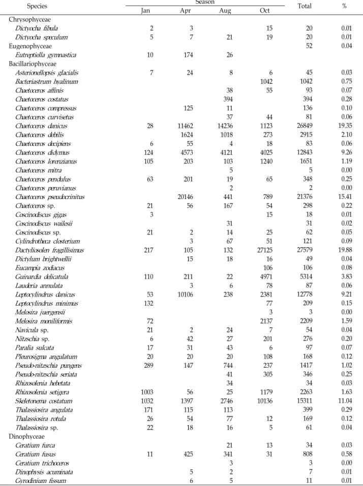
Table 1. The composition and biomass at water surface (unit: × 100 cells/l)
Species Jan Apr Season Aug Oct Total %
Chrysophyceae
Dictyocha fibula
2 3 15 20 0.01Dictyocha speculum
5 7 21 19 20 0.01Eugenophyceae 52 0.04
Eutreptiella gymnastica
10 174 26Bacillariophyceae
Asterionellopsis glacialis
7 24 8 6 45 0.03Bacteriastrum hyalinum
1042 1042 0.75Chaetoceros affinis
38 55 93 0.07Chaetoceros costatus
394 394 0.28Chaetoceros compressus
125 11 136 0.10Chaetoceros curvisetus
37 44 81 0.06Chaetoceros danicus
28 11462 14236 1123 26849 19.35Chaetoceros debilis
1624 1018 273 2915 2.10Chaetoceros decipiens
6 55 4 18 83 0.06Chaetoceros didymus
124 4573 4121 4025 12843 9.26Chaetoceros lorenzianus
105 203 103 1240 1651 1.19Chaetoceros mitra
5 5 0.00Chaetoceros pendulus
63 201 19 65 348 0.25Chaetoceros peruvianus
2 2 0.00Chaetoceros pseudocrinitus
20146 441 789 21376 15.41Chaetoceros
sp. 21 56 167 54 298 0.22Coscinodiscus gigas
3 15 18 0.01Coscinodiscus wailesii
31 31 0.02Coscinodiscus
sp. 21 2 14 25 62 0.05Cylindrotheca closterium
3 67 51 121 0.09Dactyliosolen fragillisimus
217 105 132 27125 27579 19.88Dictylum brightwellii
15 18 16 49 0.04Eucampia zodiacus
106 106 0.08Guinardia delicatula
110 211 22 4971 5314 3.83Lauderia annulata
3 6 78 87 0.06Leptocylindrus danicus
53 10106 238 2381 12778 9.21Leptocylindrus minimus
132 77 209 0.15Melosira juergensii
3 3 0.00Melosira moniliformis
72 2137 2209 1.59Navicula
sp. 21 2 24 7 54 0.04Nitzschia
sp. 6 42 27 201 276 0.20Paralia sulcata
17 31 43 6 97 0.07Pleurosigma angulatum
20 20 20 108 168 0.12Pseudo-nitzschia pungens
289 147 744 237 1417 1.02Pseudo-nitzschia seriata
41 305 346 0.25Rhizosolenia hebetata
34 34 0.03Rhizosolenia setigera
1003 56 25 1179 2263 1.63Skeletonema costatum
1032 1397 2746 10136 15311 11.04Thalassiosira angulata
171 115 113 399 0.29Thalassiosira rotula
26 54 77 12 169 0.12Thalassiosira
sp. 22 18 16 5 61 0.04Dinophyceae
Ceratium furca
21 13 34 0.03Ceratium fusus
11 425 341 31 808 0.58Ceratium trichoceros
3 3 0.00Dinophysis acuminata
5 2 7 0.01Gyrodinium fissum
6 5 11 0.01Table 1. Continued
Species Jan Apr Season Aug Oct Total %
Gyrodinium spirale
29 33 62 0.05Gyrodinium
sp. 1 2 3 0.00Heterocapsa triquetra
3 6 9 0.01Katodinium glaucum
14 19 33 0.02Noctiluca scintillans
2 2 0.00Protoperidinium bipes
3 3 0.00Prorocentrum bronchi
12 7 19 0.01Protoperidinium
sp. 3 1 2 6 0.00Protoperidinium pellucidum
11 17 28 0.02Scrippsiella trochoidea
33 56 11 100 0.07Torodinium teredo
2 2 0.00Total 3612 51531 25579 58012 138734 100
Species No. 31 42 48 41
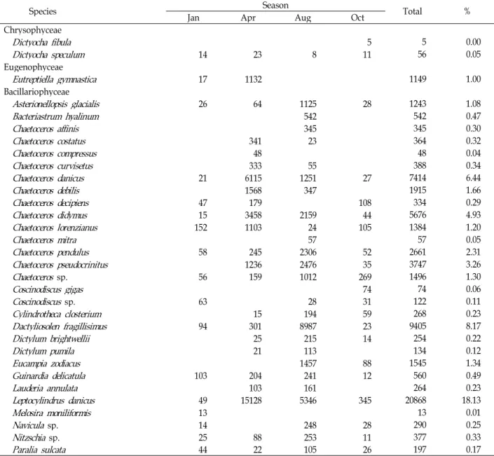
Table 2. The composition and biomass at basal layer (unit: cells/l)
Species Jan Apr Season Aug Oct Total %
Chrysophyceae
Dictyocha fibula
5 5 0.00Dictyocha speculum
14 23 8 11 56 0.05Eugenophyceae
Eutreptiella gymnastica
17 1132 1149 1.00Bacillariophyceae
Asterionellopsis glacialis
26 64 1125 28 1243 1.08Bacteriastrum hyalinum
542 542 0.47Chaetoceros affinis
345 345 0.30Chaetoceros costatus
341 23 364 0.32Chaetoceros compressus
48 48 0.04Chaetoceros curvisetus
333 55 388 0.34Chaetoceros danicus
21 6115 1251 27 7414 6.44Chaetoceros debilis
1568 347 1915 1.66Chaetoceros decipiens
47 179 108 334 0.29Chaetoceros didymus
15 3458 2159 44 5676 4.93Chaetoceros lorenzianus
152 1103 24 105 1384 1.20Chaetoceros mitra
57 57 0.05Chaetoceros pendulus
58 245 2306 52 2661 2.31Chaetoceros pseudocrinitus
1236 2476 35 3747 3.26Chaetoceros
sp. 56 159 1012 269 1496 1.30Coscinodiscus gigas
74 74 0.06Coscinodiscus
sp. 63 28 31 122 0.11Cylindrotheca closterium
15 194 59 268 0.23Dactyliosolen fragillisimus
94 301 8987 23 9405 8.17Dictylum brightwellii
25 215 14 254 0.22Dictylum pumila
21 113 134 0.12Eucampia zodiacus
1457 88 1545 1.34Guinardia delicatula
103 204 241 12 560 0.49Lauderia annulata
103 161 264 0.23Leptocylindrus danicus
49 15128 5346 345 20868 18.13Melosira moniliformis
13 13 0.01Navicula
sp. 14 248 28 290 0.25Nitzschia
sp. 25 88 253 11 377 0.33Paralia sulcata
44 22 105 26 197 0.17Table 2. Continued
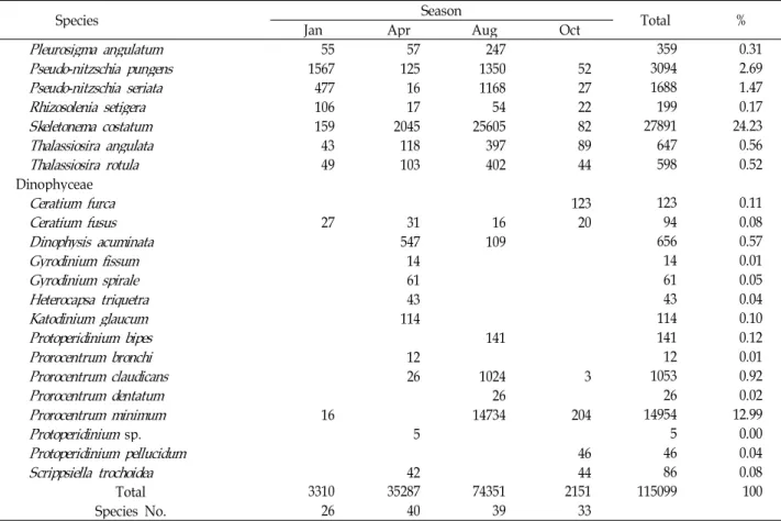
Species Jan Apr Season Aug Oct Total %
Pleurosigma angulatum
55 57 247 359 0.31Pseudo-nitzschia pungens
1567 125 1350 52 3094 2.69Pseudo-nitzschia seriata
477 16 1168 27 1688 1.47Rhizosolenia setigera
106 17 54 22 199 0.17Skeletonema costatum
159 2045 25605 82 27891 24.23Thalassiosira angulata
43 118 397 89 647 0.56Thalassiosira rotula
49 103 402 44 598 0.52Dinophyceae
Ceratium furca
123 123 0.11Ceratium fusus
27 31 16 20 94 0.08Dinophysis acuminata
547 109 656 0.57Gyrodinium fissum
14 14 0.01Gyrodinium spirale
61 61 0.05Heterocapsa triquetra
43 43 0.04Katodinium glaucum
114 114 0.10Protoperidinium bipes
141 141 0.12Prorocentrum bronchi
12 12 0.01Prorocentrum claudicans
26 1024 3 1053 0.92Prorocentrum dentatum
26 26 0.02Prorocentrum minimum
16 14734 204 14954 12.99Protoperidinium
sp. 5 5 0.00Protoperidinium pellucidum
46 46 0.04Scrippsiella trochoidea
42 44 86 0.08Total 3310 35287 74351 2151 115099 100
Species No. 26 40 39 33
ceae 15 taxa, one Cryptophyceae taxon, and one Eugenophy- ceae taxon. Diatoms and dinoflagellates were the most di- verse groups. Centric and pennate diatoms accounted for the highest diversity among of them. Results of 2 m, 4 m, 6 m, and 8 m were not shown in table and they used for water circulation analysis.
On April, a total of 40 taxa were identified at low surface layer: Bacillariophyceae 28 taxa, Dinophyceae 10 taxa, Cryptophyceae and Eugenophyceae, each of one taxon. The station C was characterized by high phytoplankton biomass.
The relative dominant species were two Dinoflagellate taxa (Chaetoceros danicus and Leptocylindrus danicus) at seven stations.
On August, a total of 39 taxa were identified at low layer:
Diatoms 32 taxa, Dinoflagellate 6 taxa. The station A was characterized by high phytoplankton biomass. The relative dominant species were three diatoms taxa (Dactyliosolen fra- gillisimus, Leptocylindrus danicus, and Skeletonema costatum) and one Dinoflagellate taxon (Prorocentrum minimum) at sev- en stations.
On October, a total of 33 taxa were identified at low layer:
Bacillariophyceae 25 taxa, Dinophyceae 6 taxa, and Crypto-
phyceae 2 taxa. The station C was characterized by high phy- toplankton biomass and station G was lowest. Leptocylindrus danicus was the most dominant species at seven stations.
Biomass
The density and biomass of species demonstrated sig- nificant patterns from the near seaside station (Stations B, C, and D) to remote seaside stations (Stations F, G). Winter season was characterized by minimum phytoplankton con- centrations and Pseudo-nitzschia pungens was dominant species. During spring season, Leptocylindrus danicus was most abundant (p<0.01) at stations A, C, and F (Table 1).
During winter season, Pseudo-nitzschia pungens was most abundant (p<0.01) at stations B and C. Skeletonema costatum was the second dominant species at station A. Rhizosolenia setigera was also abundant at station E.
During spring season, Chaetoceros pseudocrinitus was most abundant at all stations. Leptocylindrus danicus was the sec- ond dominant species. Chaetoceros danicus was also abundant at all stations. They were decreased remote seaward (p<0.01).
During summer season, Skeletonema costatum was most
abundant at all stations. Prorocentrum minimum was the sec-
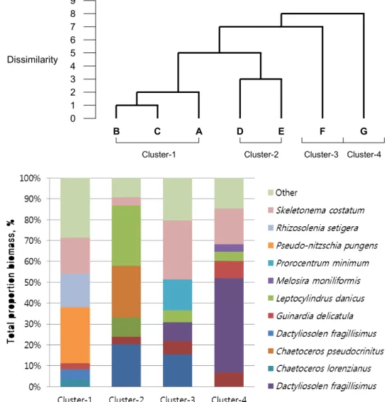
Dissimilarity 9 8 7 6 5 4 3 2 1 0
B C A D E F G
Cluster-1 Cluster-2 Cluster-3 Cluster-4
Fig. 2. Spatial variability of phytoplankton community. Upper dendrogram of the cluster analysis based on the dissimilarity among seven stations. Lowe is the compositions of dominant species in different phytoplankton associations within area outlined by the cluster analysis.
ond dominant species at the stations F and G. Chaetoceros danicus was also abundant at all stations.
During autumn season, Dactyliosolen fragillisimus was most abundant at all stations. Skeletonema costatum was the second dominant species at all stations.
Biomass of species at water surface on January was varied from 200 cells/l to 103,200 cells/l (Fig. 2). The station B was shown the highest phytoplankton density among seven stations. Biomass of species at basal layer was 1,400~156,700 cells/l and the station C was also shown the highest phyto- plankton density among seven stations.
Mean biomass of species at water surface and basal layer on April were 1,227 cells/l and 882 cells/l. Mean biomass of species at water surface and basal layer on August were 533 cells/l and 188 cells/l. Mean biomass of species at water
surface and basal layer on October were 1,415 cells/l and 65 cells/l.
Cluster analysis
Analysis of seasonal variability within the phytoplankton community was performed using the hierarchical clustering using the Jaccard Index of similarity. In the beginning of the year (January), all stations were often more than 60%
of similarity, as shown in Fig. 3. Water surface and basal
layer showed a clear distinction excluding Stations B and
C (data not shown). Stations A, B, and C formed same clus-
tered (cluster-1). They are mainly consisted of Pseudo-nitz-
schia pungens, Rhizosolenia setigera, and Skeletonema costatum
which were dominant in cluster-1 on winter. In spring, the
plankton community consisted mainly of Chaetoceros pseudoc-
Fig. 3. Simple linear regression in the phytoplankton commun- ity along an East-West longitude gradient. The vertical lines represent the SD.
Table 3. Biological diversity of phytoplankton in season at Hwadang-ri Indices
Season
Jan Apr Aug Oct
W.S. B.L. W.S. B.L. W.S. B.L. W.S. B.L.
Diversity
H` 2.246 2.114 1.700 2.056 1.639 2.255 1.875 3.023
N1 9.449 8.274 5.472 7.815 5.148 9.536 6.521 20.552
N2 5.672 3.930 3.992 4.298 2.852 5.476 3.757 14.395
Richness
R1 3.662 3.085 3.779 3.725 4.631 3.388 3.647 4.170
R2 0.516 0.452 0.185 0.213 0.300 0.143 0.170 0.712
Evenness
E1 0.654 0.649 0.455 0.557 0.423 0.616 0.505 0.865
E2 0.305 0.318 0.130 0.195 0.107 0.245 0.159 0.623
E3 0.282 0.291 0.109 0.175 0.088 0.225 0.138 0.611
E4 0.600 0.475 0.729 0.55 0.554 0.574 0.576 0.7
E5 0.553 0.403 0.669 0.484 0.447 0.524 0.499 0.685
Table 4. Space-time variability of the phytoplankton community structure
Attributes of community structure Spatial variability (7 stations) Temporal variability (4 seasons) Water surface Basal Layer Water surface Basal Layer Mean number of species per sample
Number of species with absolute occurrence Number of samples containing all species Occurrence index (β-diversity)
28 127 1.481
25 58 1.125
41 1122 1.725
35 1619 1.347
rinitu and Leptocylindrus danicus (Cluster-2). Relative remote
stations (F and G) were characterized by low similarity be- tween stations or two layers in depths and minimal values of species diversity and community evenness. In late au- tumn, the phytoplankton community consisted mainly of Skeletonema costatum and Pseudo-nitzschia pungens.
Spatial and temporal variability of phytoplankton Water surfaces were shown with the relative individual density or abundance across areas (Table 1 and Table 2).
However, Shannon-Weaver indices of diversity of water sur- faces were lower than those of basal layers except January (Table 3). In addition, evenness indices of basal layers were higher than those of water surfaces except January.
The station A had high number of species as well as those of both area, B and C (data not shown). Shannon-Weaver index of diversity also varied among the stations and season with 3.023 (October) and 2.255 (August) having higher value than the other stations and season.
Assessments of the seven spatial and four seasonal varia- bility of the structure of the phytoplankton community were presented in Table 4. Although the numbers of species with absolute occurrence were existed in stations and season, mean paired similarity between both the species composi- tion within stations and within seasons were high levels.
For the community as a whole, the values of ß-diversity
were the low (1.125 for water surface within seven stations
and 1.481 for basal layer) or common (1.725 for water surface
within four seasons and 1.347 for basal layer). They in-
dicated that heterogeneity in species compositions among
Table 5. Test of homogeneity of the phytoplankton community between the four seasons at Hwadang-ri
Month January April August October
January April August October
- 0.159 (32) 0.794 (45) 1.927 (44)
p
>0.05 0.211 (37)- 0.223 (39)p
>0.05p
>0.05- 0.084 (44)
p
>0.05p
>0.05p
>0.05- Upper diagonal is the degree of significant for
p
value and low diagonal ist
value. Parenthesis is the degree of freedom.Table 6. Test of homogeneity of the phytoplankton community between the seven stations at Hwadang-ri
Station A B C D E F G
A B DC EF G
- -0.038
0.210 3.149 3.237 3.547 3.268
p
>0.05 - 0.222 2.320 2.531 3.015 2.854p
>0.05p
>0.05 1.815- 2.536 2.731 2.711p
<0.01p
<0.05p
>0.05- 1.962 2.611 2.477
p
<0.01p
<0.05p
<0.05p
>0.05 1.685- 1.608p
<0.01p
<0.01p
<0.01p
<0.01p
>0.05- -0.084
p
<0.01p
<0.01p
<0.01p
<0.01p
<0.05p
>0.05- Upper diagonal is the degree of significant for
p
value and low diagonal ist
value.Distance (× 170 m)
Fig. 4. Percentage contribution of phytoplankton groups to the total species richness plotted against geographical distances.
the replicates were not high. The parameters paired sim- ilarity between season and stations testified (Table 5). There were high taxonomic homogeneity of the phytoplankton community in between four seasons and similar trends in seasonal development of phytoplankton at depths of same stations. However, size distribution of abundance and bio- mass showed a statistically significant west-east different (p
<0.05, Table 6).
In order to assess macro-scale spatial variability of the phytoplankton community at Hwadang-ri, I analyzed dis- tributions of species richness and diversity of large taxo- nomic groups as well as phytoplankton composition along a longitudinal gradient. Figure 3 showed the biomass plotted against longitude. Margalef’s index gradually decreased from west to east. This trend conformed to a linear re- gression model, which described 85% of the spatial varia- bility for mean species biomass (r
2=0.67).
Phytoplankton composition from western areas near the Hwadang-ri was more diverse than that of eastern areas.
This decreasing trend was supported mainly by an increase of phytoplankton diversity. The mean number of species within the western waters was 55 taxa and eastern was 44.
The portion of dinoflagellates in the phytoplankton de- creased exponentially along the west-east gradient (Fig. 4).
The diatom/dinoflagellate ratio was equal to 0.768 within western waters (Stations A, B, C); whereas it was reduced to 0.894 in middle waters, and even further to 1.044 in open waters.
Discussion
Diatoms dominated phytoplankton abundance numeri-
cally as well as in biomass, accounting for 98.98% of the
latter depending on season. Phytoplankton concentrations,
which were obtained in this study, are within the range of
those reported previously [2]. Both the spatial and temporal
components contributed to the variability of the phyto-
plankton community at Hwadang-ri in Goseng-gun. During
the winter months, the western area was characterized by
the lowest concentrations of phytoplankton. It was strongly
correlated with temperature from cold river introduction of
inland, whereas the highest phytoplankton concentrations
were observed in open waters. The minimum diversity level
was associated with the winter months, whereas the max- imum was in autumn (October). Phytoplankton species rich- ness gradually increased eastward, with the lowest richness recorded in the waters closest to the coastal-side (Stations A, B, C) and the highest towards the eastern waters (Stations F, G). These east-west differences in the phytoplankton com- munity have been reported for the Pacific [4, 10, 16]. This east-west difference in the phytoplankton community may reflect heterogeneity in the grazing pressure of the zoo- plankton community [9, 19] or temperature and magnitude of the spring phytoplankton bloom [21].
Most of the time, marine waters are characteristically blue or green and reasonably clear. In the temperate waters of the northern latitudes, water is seldom as clear as seen in tropical areas, where visibility can exceed 50-75 feet [22]. In temperate waters, the limits of visibility or murkiness are usually the result of algae in the water. However, in some unusual cases, a single microalgal species can increase in abundance until they dominate the microscopic plant com- munity and reach such high concentrations that they dis- color the water with their pigments, these “blooms” of algae are often referred to as a “Red tide”. Although referred to as Red tides, blooms are not only red, but can be brown, yellow, green, or milky in color [7]. Adverse effects can like- wise occur when algal cell concentrations are low and these cells are filtered from the water by shellfish such as clams, mussels, oysters, scallops, or small fish. Many animals at higher levels of the marine food chain are impacted by harmful algal blooms. Toxins can be transferred through successive levels of the food chain, sometimes having lethal effects.
Euglenophyceae (Eutreptiella gymnastica) was found in the four stations on January and the all stations on April in this study (Table 1 and Table 2) to be the major bloom formers [7]. Chaetoceros curvisetus, Leptocylindrus danicus, Skeletonema costatum, Cylindrotheca closterium, Pseudo-nitzschia pungens, Navicula spp. of Bacillariophyceae were also found in most stations and seasons to be the major bloom formers [7].
Ceratium furca, Ceratium fusus, Gyrodinium fissum, Heterocapsa triquetra, Prorocentrum dentatum, Prorocentrum minimum, Scrippsiella trochoidea of Dinophyceae were found to be the major bloom formers.
We expect that this work may provide valuable in- formation of interest to later ecological studies. Definitive identification of the principal phytoplankton species as- sumes greater importance also at the light of the potentially
serious and harmful effects associated with bloom events.
Acknowledgement
This work was supported by Dong-eui University Grant (2014AA472).
References
1. Almandoz, G. O., Hernando, M. P., Ferreyra, G. A., Schloss, I. R. and Ferrario, M. E. 2011. Seasonal phytoplankton dy- namics in extreme southern South America (Beagle Channel, Argentina).
J Sea Res
66, 47–57.2. Al-Zaidan, A. S. Y., Kennedy, H., Jones, D. A. and Al-Mohanna, S. Y. 2006. Role of microbial mats in Sulaibikht Bay (Kuwait) mudflat food webs: evidence from δ13C analysis.
Marine Ecology Progress Series
308, 27–36.3. Falkowski, P. G., Laws, E. A., Barber, R. T. and Murray, J. W. 2003. Phytoplankton and their role in primary, new, and export production, pp. 99-121. In: Fasham, M. J. R. (ed.),
Ocean biogeochemistry: This Role of the Ocean Carbon Cycle in Global Change
. Springer, Berlin, Heidelberg, NY.4. Harrison, P. J., Boyd, P. W., Varela, D. E., Takeda, S., Shiomoto, A. and Odate, T. 1999. Comparison of factors con- trolling phytoplankton productivity in the NE and NW sub- arctic Pacific gyres
. Prog Oceanogr
43, 205–234.5. Hill, M. O. 1973. Diversity and evenness: a unifying notation and its consequences.
Ecology
54, 423-432.6. IBM Corp. Released 2012.
IBM SPSS Statistics for Windows
,Version 21.0.
Armonk, NY: IBM Corp.7. Lee, D. K. 2008.
Cochlodinium polykriklides
blooms and eco- physical conditions in the South Sea of Korea.Harmful Algae
7, 318-323.8. Lee, S. G., Kim, H. G., Bae, H. M., Kang, Y. S., Jeong, C.
S., Lee, C. K., Kim, S. Y., Kim, C. S., Lim, W. A. and Cho, U. S. 2002.
Handbook of Harmful Marine Algal Blooms in Korean Waters,
pp. 172, National Fisheries Research and Develop- ment Institute, Republic of Korea, Seoul.9. Mackas, D. L. and Tsuda. A. 1999. Mesozooplankton in the eastern and western subarctic Pacific: community structure, seasonal life histories, and interannual variability.
Prog Oceanogr
43, 335–363.10. Magurran, A. E. 1988.
Ecological diversity and its measurement,
pp. 192, Princeton Univ. Press, Cambridge, USA.11. Matsuno, K. and Yamaguchi, A. 2010. Abundance and bio- mass of mesozooplankton along north-south transects (165°E and 165°W) in summer in the North Pacific: an analy- sis with an optical plankton counter.
Plankton Benthos Res
5, 123-130.12. McWilliams, J. C. 1996. Modeling the oceanic general circulation.
Annu Rev Fluid Mech
28, 215-248.13. Merritt, R. W. and Cummins, K. W. 1996.
An Introduction
to the Aquatic Insects of North America,
pp. 862, 3rd ed., Kendall/Hunt., Dubuque, Iowa.초록:고성군 화당리 연안에서 식물플랑크톤의 계절 및 지점별 조성 변화 강만기
1․허만규
2*
(
1동의대학교 자연 ․생활과학대학 데이터정보학과,
2동의대학교 자연 ․생활과학대학 분자생물학과)
본 연구는 2013년 고성군 화당리에 있는 7개 지점에 대한 식물 플랑크톤의 공간적 분포, 계절적 분포, 표층과
심층의 깊이에 따른 빈도에 대해 기술한 것이다 . 화당리에서 식물 플랑크톤 군집은 3강 60분류군으로 다양하였다.
규조강 (Bacillariophyceae)은 41분류군으로 가장 높은 다양성을 나타내었으며 그 다음으로는 와편모강(Dinophy- ceae)으로 16분류군이었고, 황금색조식물강(Cryptophyceae)이 2분류군, 유글레나식물강(Eugenophyceae)이 1분류
군이었다 . 표층은 비교적 높은 밀도와 풍부도를 유지하고 있었다. 그런데 Shannon-Weaver의 다양도 지수는 1월
을 제외하고는 표층보다 저층에서 더 높았다 . 또 균등도 지수도 1월을 제외하고는 표층보다 저층에서 더 높았다.
전체 군집에 대해 ß-다양도는 낮거나(7개 정점의 공간적 표층은 1.125, 저층은 1.481) 보통(7개 정점의 시간적 표층
은 1.725, 저층은 1.347)이었다. 계절에 따라서는 식물 플랑크톤의 군집 간에 분류학적 동질성이 있었다. 깊이에
대해서도 역시 동질성을 나타내었다 . 그러나 풍부도의 분포와 생체량은 동-서 방향 구배가 유의한 차이를 나타내
었다 .
14. Pielou, E. C. 1966. The measurement of diversity in different types of biological collection.
J Theoret Biol
13, 131-144.15. Shannon, C. E. and Weaver, W. 1963.
The Measurement Theory of Communication,
pp. 1-117, Univ. of Illinois Press, Urbana, USA.16. Shiomoto, A. and Hashimoto, S. 2000. Comparison of east and west chlorophyll
a
standing stock and oceanic habitat along the transition domain of the North Pacific.J Plankton Res
22, 1-14.17. Sournia, A. 1978.
Phytoplankton manual. In Monographs on Oceanographic Methodology 6
, pp. 337, UNESCO, Paris.18. Stanca, E., Roselli, L. Cellamare, M. and Basset, A. 2013.
Phytoplankton composition in the coastal Magnetic Island lagoon, Western Pacific Ocean (Australia) TWB, Transit.
Waters Bull
7, 145-158.19. Takahashi, K., Kuwata, A., Saito, H. and Ide, K. 2008.
Grazing impact of the copepod community in the Oyashio region of the western subarctic Pacific Ocean.
Prog Oceanogr
78, 222-240.20. Tomas, C. R. 1997.
Identifying marine phytoplankton. Academic press,
pp. 858, Harcourt Brace and Company, Toronto.21. Tsuda, A., Saito, H. and Kasai, H. 2004. Life histories of
Eucalanus bungii
andNeocalanus cristatus
(Copepoda:Calanoida) in the western subarctic Pacific Ocean.
Fish Oceanogr
13, 10-20.22. Verlencar, X. N. 2004.
Phytoplankton Identification Manual
, pp.1-40, National Institute of Oceanography, Dona Paula, India.
23. Wiederholm, T. 1983.