Goodness-of-fit tests for a proportional odds model

Goodness-of-fit tests for a proportional odds model

Hyun Yung Lee ¹

1 Department of Information Statistics, Kyung-Sung University

Received 29 June 2013, revised 7 August 2013, accepted 30 August 2013

Abstract

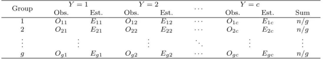
The chi-square type test statistic is the most commonly used test in terms of mea- suring testing goodness-of-fit for multinomial logistic regression model, which has its grouped data (binomial data) and ungrouped (binary) data classified by a covariate pattern. Chi-square type statistic is not a satisfactory gauge, however, because the ungrouped Pearson chi- square statistic does not adhere well to the chi-square statis- tic and the ungrouped Pearson chi-square statistic is also not a satisfactory form of measurement in itself. Currently, goodness-of-fit in the ordinal setting is often assessed using the Pearson chi-square statistic and deviance tests. These tests involve creat- ing a contingency table in which rows consist of all possible cross-classifications of the model covariates, and columns consist of the levels of the ordinal response. I exam- ined goodness-of-fit tests for a proportional odds logistic regression model-the most commonly used regression model for an ordinal response variable. Using a simulation study, I investigated the distribution and power properties of this test and compared these with those of three other goodness-of-fit tests. The new test had lower power than the existing tests; however, it was able to detect a greater number of the different types of lack of fit considered in this study. I illustrated the ability of the tests to detect lack of fit using a study of aftercare decisions for psychiatrically hospitalized adolescents.

Keywords: Goodness-of-fit, Hosmer-Lemeshow test, ordinal logistic regression, ordinal models, ordinal response, proportional odds.

1. Introduction

An ordinal logistic regression model describes the relationship between an ordinal response variable (from low to high)-such as the level of the fear of crime classified as not at all fearful, not very fearful, somewhat fearful, or very fearful-and one or more explanatory variables (covariates). It is different from the multinomial logistic regression model, which does not take the ordering of the response categories into account. Several different ordinal models can be used: the proportional odds, the constrained and unconstrained partial-proportional odds, the adjacent-category, the continuation-ratio, and the stereotype logistic models (Hosmer and Lemeshow, 2000; Agresti, 2010). The most frequently used model is the proportional odds model, also called the (constrained) cumulative logit or the parallel-lines model. It is available in most general purpose statistical software packages, such as SAS. Lee (2012)

1

Assistant professor, Department of Information Statistics, Kyung-Sung University, Pusan 608-736,

Korea. E-mail: [email protected]

compared the estimators of parameters in the GEE approach for the ordinal response and Kim and Lee (2013) also discussed about proportional hazard model.

All regression models for categorical response variables should be evaluated for fit and their adherence to model assumptions. The test by Hosmer-Lemeshow (1980) is available in most software packages and has gained widespread use.

For ordinal regression models, few methods exist to assess goodness-of -fit, and no general goodness-of-fit test is widely available in software packages. Lipsitz et al . (1996) proposed a goodness-of-fit test, partly based on the Hosmer-Lemeshow approach, for a general or- dinal regression model. The test provides no contingency table of observed and estimated frequencies and is not always computable for small sample sizes. Pulkstenis and Robinson (2004) modified the Pearson chi-square and deviance statistics so that they could be used for testing goodness-of-fit in ordinal models that include continuous covariates. One limitation with that approach was that the regression model needed to include both continuous and categorical covariates.

Also, if many categorical covariates were present, the performance of the tests may suffer because of the large number of cells from which the Pearson chi-square and deviance statistics were calculated.

The purpose of this paper is to present a new goodness-of-fit test for the proportional odds model. I used the approach first suggested by Hosmer and Lemeshow (1980) to partition the data into suitable groups. In Section 3, I cross-classified the groups with the response categories and test goodness of-fit using the Pearson chi-square statistic on the resulting table of observed and estimated frequencies. One benefit of using the Hosmer-Lemeshow method was that I could now assess goodness-of-fit using the same approach for binary, multinomial, and ordinal logistic regression models. In Section 4, I investigated the power of the new test and compare it with the tests by Lipsitz et al . (1996) and Pulkstenis and Robinson (2004). I used a study of determinants of aftercare placement for psychiatrically hospitalized adolescents (Fontanella, 2008) to illustrate the application of the tests.

2. The proportional odds model

Let Y denote an ordinal response variable with c levels (1, · · · , c), and let x be a vector of p explanatory variables, from now on called covariates. The proportional odds model compares the probability of an equal or smaller response (Y ≤ j) with the probability of a larger response (Y > j), both conditional on the covariates, through c − 1 logits

g j (x) = log

"

P (Y ≤ j|x) P (Y > j|x)

#

(2.1)

= α j + β 1 x 1 + · · · + β p x p , j = 1, · · · , c − 1.

The regression coefficients β 1 , · · · , β p are constant across the logits, whereas the intercepts are such that α 1 < α 2 < · · · < α c−1 . It follows from (2.1) that

P (Y ≤ j|x) = e ^g

^(x)

1 + e ^g

^(x) , j = 1, · · · , c − 1. (2.2)

Let π _j = P (Y = j|x) denote the conditional probability of a response equal to j given x.

It follows from (2.2) that

π ₁ = P (Y ≤ 1|x),

π j = P (Y ≤ j|x) − P (Y ≤ j − 1|x), j = 2, · · · , c − 1 and

(2.3)

π c = 1 − P (Y ≤ c − 1|x).

Suppose that I have a sample of n independent observations, denoted by (x i , y i ), i = 1, · · · , n. Let π ij = P (Y = j|x i ). For notational simplicity, let ˜ y ij denote binary indicator variables, such that ˜ y ij = 1 if y i = j and ˜ y ij = 0 given that (i = 1, · · · , n; j = 1, · · · , c).

The proportional odds model may be fitted and estimates of α and β calculated by standard maximum likelihood methods (Hosmer and Lemeshow, 2000; Agresti, 2010). Following the fit of the model, I denote the estimated probabilities of each response level for each observation as b π ij .

3. Derivation of test statistics

3.1. Lipsitz test

Lipsitz et al . (1996) proposed a goodness-of-fit test for ordinal regression models, includ- ing the proportional odds model. Suppose that the estimated probabilities b π _ij have been calculated from a fitted ordinal regression model, an ordinal score to each observation is assigned using equally spaced integer weights:

s _i = b π _i1 + 2 b π _i2 + · · · + c b π _ic , i = 1, · · · , n. (3.1) The observations are organized into g groups based on the ordinal score s _i , such that group 1 contains the n/g observations with the lowest scores and group g contains the n/g observations with the highest scores. Create g − 1 binary indicator variable I _k , such that

I ik =

( 1 if observation i is in group k 0 otherwise

for i = 1, · · · , n and k = 1, · · · , g − 1. A new ordinal regression model is fitted that includes indicator variables:

g j (x) = α j + β 1 x 1 + · · · + β p x p + γ 1 I 1 + · · · + γ g−1 I g−1 , j = 1, · · · , c − 1. (3.2) When the fitted model is the correct model, γ 1 = 0, · · · , γ g−1 = 0. Let L 1 and L 0 denote the log likelihoods of the fitted models (2.1) and (3.2), respectively. A goodness-of-fit test is obtained by comparing the value of the likelihood ratio statistic −2(L 1 − L 0 ) with the chi-square distribution with g − 1 degrees of freedom. Lipsitz et al . (1996) suggested that the number of groups should be chosen such that 6 ≤ g < n/5c. I refer to the test as the Lipsitz test.

Lipsitz et al . (1996) also suggested, but did not illustrate, using scores s _i = b π _i1 . They

pointed out that since π b ₁ was a monotone function of the linear predictor, this grouping was

equivalent to a grouping based on b βx. Lipsitz et al . (1996) also pointed out that under the null hypothesis, their test was a linear combination of the differences (O _kj − E _kj ),

O _kj = X

l∈Ω

y e _lj (3.3)

E kj = X

l∈Ω

b π lj (3.4)

for k = 1, · · · , g, j = 1, · · · , c, and where Ω _k denotes indices of the n/g observations in group k.

3.2. Pulkstenis and Robinson tests

If only categorical covariates are present, I can construct a contingency table of observed and estimated frequencies, where the rows consist of all possible covariate patterns and the columns represent the response levels. Goodness-of-fit can then be assessed using the Pearson chi-square and deviance statistics. When continuous covariates are present, this approach fails because the number of covariate patterns approaches (or is equal to) n, the sample size, making the contingency table sparsely populated.Pulkstenis and Robinson (2004) suggested an extension of the Pearson chi-square and deviance statistics that allowed continuous covariates. First, the covariate patterns using the categorical covariates only were determined and any unobserved patterns were disregarded. The ordinal score (3.1) was calculated and each covariate pattern was split into two on the basis of the median ordinal score within each pattern. A table of observed and estimated frequencies was constructed based on the cross-classification of covariate patterns with response levels. From this table, the modified Pearson chi-square and deviance statistics are obtained as

χ ² =

2

X

l=1 K

X

k=1 c

X

j=1

(O lkj − E lkj ) ²

E _lkj (3.5)

and

D ² = 2

2

X

l=1 K

X

k=1 c

X

j=1

O _lkj log O lkj

E lkj

(3.6)

where l indexes the two subgroups based on the ordinal scores, K is the number of observed covariate patterns due to the categorical covariates, and c is the number of response levels.

The reference distribution for both statistics is the χ ² distribution with (2K − 1)(c − 1) − p _cat − 1 degrees of freedom, where p _cat is the number of categorical covariates. For example, if one fits a model with three dichotomous covariates and one covariate with five levels modeled with four design variables, then p _cat = 7. I refer to the two tests defined by (3.5) and (3.6) as the PR(χ ² ) and PR(D ² ) tests and collectively as the Pulkstenis-Robinson (PR) tests.

3.3. Proposed test statistic

The test I proposed in this paper was based on an approach first suggested by Hosmer

and Lemeshow (1980) for binary logistic regression and later adapted to multinomial logistic

regression by Fagerland et al . (2008). In the binary setting (Y = 0, 1), following the fit of the model, the observations were grouped according to the estimated probabilities of Y = 1.

Usually, 10 groups were formed, often called the deciles of risk. However, the number of groups (g) could be arbitrary. Within each group, the number of observed and estimated frequencies were summed, both for Y = 0 and Y = 1. A g × 2 contingency table containing the observed and estimated frequencies could be constructed. The test statistic is the Pear- son chi-square statistic from that table, and the reference distribution was the chi-square distribution with g − 2 degrees of freedom (Hosmer and Lemeshow, 1980).

Similarly, after fitting a multinomial logistic regression model (Y = 0, · · · , c − 1), the observations are arranged into g groups by the estimated probabilities 1 − b π i0 which has the complement of the estimated probability of the reference response category (Y = 0). The observed and estimated frequencies in each group for each response level may be summarized in a contingency table, now with g rows and c columns. The multinomial test statistic was the Pearson chi-square statistic from this table, and the reference distribution was the chi-square distribution with (g − 2)(c − 1) degrees of freedom (Fagerland et al ., 2008).

I proposed a similar approach for the proportional odds model. After calculating the es- timated probabilities π b _ij , I computed the ordinal scores (3.1). As for the binary and multi- nomial settings, I partitioned the observations into g groups, this time based on the ordinal score, such that group 1 contained the n/g observations with the lowest scores and group g contains the n/g observations with the highest scores. As noted in Section 3.1, sorting according to the ordinal score is identical to sorting according to 1 − π b i1 . The score was used to sort and group the observations in the multinomial test (Fagerland et al., 2008).

The observed and estimated frequencies in each group for each response level were denoted by O kj and E kj , respectively, as defined in (3.5) and (3.6). Table 3.1 displays the sums of the observed and estimated frequencies. The ordinal test statistic is the Pearson chi-square statistic given by

T _g =

g

X

k=1 c

X

j=1

(O kj − E kj ) ²

E _kj . (3.7)

I added additional degrees of freedom to the (g − 2)(c − 1) of the multinomial test to reflect the fact that the sum of the estimated frequencies was not equal to the observed frequencies in each of the c levels of the response. The overall sums of the estimated frequencies and the observed ones were equal. One additional degree of freedom is lost because of the rank ordering constraint on the intercepts. Thus, I posited that the degrees of freedom for the ordinal test were (g − 2)(c − 1) + (c − 2).

Table 3.1 Observed (O

) and estimated (E

) frequencies sorted and summed into g groups

Group Y = 1 Y = 2

· · · Y = c

Obs. Est. Obs. Est. Obs. Est. Sum

1 O

E

O

E

· · · O

E

n/g

2 O

E

O

E

· · · O

E

n/g

. .

. . . . . . . . . . . . . . . .

g O

E

O

E

· · · O

E

n/g

As the grouping of the observations was based on estimated probabilities, the regression

models needed to have at least as many covariate patterns as the number of groups (g)

for the T _g test to work. I achieved this when there were continuous covariates or several categorical covariates present. I could assess the fit of models with, for instance, only one, two, or three dichotomous covariates with the Pearson chi-square and deviance statistics as i’ve explained in the first paragraph of Section 3.2.

4. Assessing the power of the tests

For the simulations used to check the null distribution of the test statistics, I considered models with three levels of the response. I designed the simulation study in order for it to assess the possible effects of sample size (n), covariate distribution, and number of response levels (c). Three sample sizes were used: n = 100, 150and200. Let x denote a continuous covariate. In all simulation settings, I distributed x as N (5, 3). Let d denote a dichotomous covariate distributed as Bernoulli(0.5). I used min(10, n/5c) as the number of groups for three T g tests: T 8 , T 10 andT 12 . The number of simulated replications was 10,000 throughout.

And I used 5,000 simulated replications. I outlined the power for two different situations as outlined in Sections 4.1-4.2.

4.1. Wrong functional form of a continuous covariate

I generated a three-level response variable from the following proportional odds model g _j (x) = α _j − 0.25e ^x + 0.5d, j = 1, 2, (4.1) whereas the fitted model included the term x instead of e ^x . The intercepts were α _j = [0.0, 2.0].

4.2. Omission of an interaction term between a continuous and a dichotomous covariate

I generated a three-level response variable from the following proportional odds model g j (x) = α j − 0.25x − 1.0d + β 3 xd, j = 1, 2, (4.2) where the fitted model excluded the interaction term (β 3 = 0). The intercepts were α j = [0.0, 2.0]. The coefficient β 3 was 0.3 and 0.4, corresponding to an increasing difference be- tween the correct and fitted models.

4.3. Summary of the power results

When the proportional odds model was fitted with an x term instead of the correct e ^x term. The empirical powers for the model (4.1) with wrong functional form are presented in Table 4.1. The power of the proposed statistic T g for the model (4.1) with wrong functional form is about 30% and 40% at α = 0.05, α = 0.10, respectively. The powers of all tests increase accordig to the sample sizes.

The power to detect a missing interaction term, both between a continuous and a dichoto-

mous covariate and between two dichotomous covariates, is presented in Table 4.2. The

power of the proposed statistic T _g has greater power than the PR tests exept PR(D ² ). All

the tests have a power greater than 20% for large sample sizes.

Table 4.1 Power (%) for the detection of a wrong functional form when x is normally distributed

n=100 n=150 n=200

Significance level 5% 10% 5% 10% 5% 10%

T

23.0 35.0 31.5. 41.0 33.5 44.5

T

23.4 31.4 32.6 42.2 33.7 45.4

T

24.0 32.0 33.0 42.5 33.9 46.1

PR(χ

) 10.5 22.0 17.5 27.0 19.5 46.5

PR(D

) 20.5 27.0 29.5 40.0 30.0 27.5

Table 4.2 Power (%) for the detection of a missing interaction term between a continuous and a dichotomous covariate when x is normally distributed and β

= 0.4

n=100 n=150 n=200

Significance level 5% 10% 5% 10% 5% 10%

T

15.0 27.0 20.5 31.0 24.0 37.0

T

14.9 26.5 19.0 29.9 23.0 36.5

T

14.4 26.0 18.5 29.5 22.5 35.5

PR(χ

) 10.5 22.0 16.0 26.5 21.0 39.0

PR(D

) 17.0 31.5 27.5 38.5 33.5 46.5

5. Clinical example: Determinants of aftercare placement

Hosmer et al . (2013) considered ordinal models in some detail and illustrated fitting the proportional odds model with data from a study reported by Fontanella et al . (2008) on the influence of clinical and nonclinical factors based on the decision about aftercare services for psychiatrically hospitalized adolescents. The medical records of 508 adolescents admitted to three psychiatric hospitals were collected, which included sociodemographics, clinical and family characteristics, service history, and treatment characteristics.

Table 5.1 Results of fitting a proportional odds model of neuro on age, age

, gender, race, emot and cust; n=508

df Coefficient Standard error Wald Chi-Square Pr > |z|

Age 1 1.9733 0.8646 5.2095 0.0225

Age

1 -0.0687 0.0299 5.2790 0.0216

Gender 1 0.1589 0.0975 2.6579 0.1030

Race 1 0.1842 0.0974 3.5764 0.0586

Emot 1 -0.6723 0.2227 9.1133 0.0025

Cust 1 0.5906 0.2076 8.0945 0.0044

α b

1 -13.2021 6.1815 4.5614 0.0327

α b

1 -12.2333 6.1774 3.9218 0.0477

α b

1 -11.6750 6.1742 3.5734 0.0587

Table 5.2 Observed and estimated frequencies sorted according to the ordinal score and summed into 10 groups, following the fit in Table 5.1

Group Neuro=1 Neuro=2 Neuro=3 Neuro=4

Obs. Est. Obs. Est. Obs. Est. Obs. Est. Sum

1 42 42.5 7 4.88 1 1.47 1 2.12 51

2 40 40.2 8 6.09 1 1.91 2 2.82 51

3 37 39.0 9 6.66 1 2.13 4 3.19 51

4 38 37.3 7 7.46 1 2.47 5 3.77 51

5 42 35.8 4 7.68 2 2.59 2 4.98 50

6 35 35.5 10 8.26 2 2.84 4 4.42 51

7 28 33.6 12 9.03 4 3.23 7 5.16 51

8 35 32.1 4 9.58 6 3.53 6 5.78 51

9 26 29.2 12 10.5 5 4.14 8 7.11 51

10 27 23.7 8 11.4 6 5.10 9 9.83 50

Here, I considered only a subset of the variables from that study, and I did not aim to give a complete assessment of the factors that influenced aftercare placement. I used a model from these data to illustrate the application of the goodness-of-fit tests under study in this paper, and the results I provided should be interpreted in that perspective.

First, I fit a proportional odds model using Neuro (neuropsychiatric disturbance: 1=none, 2=mild, 3=moderate, 4=severe) as the response variable and Age (in years, centered about the sample mean age of 14.3 years), Age ² (centered about the mean age), Gender (0=fe- male, 1=male), Race (0=white, 1=non-white), Emot (emotional disturbance: 0=mild, 1=

severe), and Custd (state custody: 0=no, 1=yes) as covariates. I gave the results in Table 5.1. The results showed that gender, race, emotional disturbance, and not being in state custody were associated with more severe neuropsychiatric disturbance. The effect of the model being quadratic in age was that the age at minimum odds of more severe neuropsy- chiatric disturbance is close to the average age of 14.3 years, and it increased for children younger or older. I calculated the T _g test using 10 groups and obtained p = 0.73. I gave the contingency table of observed and estimated frequencies in Table 5.2. Neither the p-value nor an assessment of the contingency table indicated lack of fit. After calculating the Lipsitz (p = 0.45) and the test by Pulkstenis and Robinson (p = 0.62 and p = 0.39), I found no evidence of lack of fit for this model.

Table 5.3 Results of fitting a proportional odds model of danger on age, gender, los, behave and elope; n = 508

df Coefficient Standard error Wald Chi-Square Pr > |z|

Age 1 0.0850 0.0524 2.6306 0.1048

Gender 1 0.2827 0.0943 8.9926 0.0027

LOS 1 -0.00631 0.00282 5.0032 0.0253

Behave 1 -0.5982 0.0546 119.8610 <.0001

Elope 1 0.3211 0.1854 2.9981 0.0834

α b

1 -0.4812 0.8242 0.3409 0.5593

α b

1 1.3564 0.8237 2.7116 0.0996

α b

1 2.8941 0.8359 12.1305 0.0005

Table 5.4 Observed and estimated frequencies sorted according to the ordinal score and summed into 10 groups, following the fit inTable 5.3

Group Danger=1 Danger=2 Danger=3 Danger=4

Obs. Est. Obs. Est. Obs. Est. Obs. Est. Sum

1 28 24.8 15 18.0 0 6.06 8 2.06 51

2 16 11.4 18 21.2 7 12.8 10 5.59 51

3 5 6.64 18 18.0 18 16.8 10 9.59 51

4 3 4.48 17 14.7 16 18.3 15 13.5 51

5 1 2.88 11 11.0 19 18.2 19 18.0 50

6 1 2.23 11 9.14 18 17.7 21 21.9 51

7 0 1.63 5 7.11 16 16.2 30 26.0 51

8 0 1.14 4 5.25 17 14.0 30 30.7 51

9 0 0.73 2 3.51 21 10.8 28 35.9 51

10 0 0.39 0 1.93 9 6.78 41 40.9 50

As a second example, I considered the response variable Danger (danger to others; 1=Un-

likely, 2=Possibly, 3=Probably, and 4=Likely), which was an assessment of the danger the

patients posed to others. In table 5.3, I fit a proportional odds model to Danger using Age (not centered), Gender, LOS (length of stay in hospital, days), Behave (behavioral symp- tom score 0-9), and Elope (elopement risk; 0=no risk, 1=history of risk) as covariates. The results showed that gender, age and elopement risk were associated with greater risk of danger to others, whereas decreasing length of stay and behavior score were associated with decreasing risk of danger to others. However, before one uses any fitted model for inferential purposes, one must evaluate fit and model assumptions. I calculate the goodness-of-fit tests and obtained a value of p = 0.0004 with the T 10 test, p = 0.54 with the Lipsitz test, and p = 0.0051 and p = 0.0056 with the PR tests. The T 10 test indicated lack of fit due to sev- eral large differences between observed and estimated frequencies (Table 5.4), a result that was supported by the two PR tests. After fitting an unconstrained continuation-ratio model (Hosmer and Lemeshow, 2000), which did not assume independence of covariate effects and response categories, I observed variation across logits for several of the coefficients (data not shown). The assumption of proportional odds thereby did not seem to be satisfied for the fitted model in Table 5.3. At this point, one might continue using the unconstrained model.

The goodness-of-fit tests discussed here have not, as yet, been extended to this model.

I noted one issue concerning the size of the estimated frequencies. Lipsitz et al . (1996) suggested that all E kj s should be greater than 1 and at least 80% should be greater than 5 for the 2-approximation to hold. In the Lipsitz test, the number of groups was chosen such that 6 ≤ g < n/5c, making the average E kj greater than 5, thus slightly reducing the problem. In the tests by Pulkstenis and Robinson (2004), the number of groups was based on the number of categorical covariate patterns. When there were many categorical covariates, the number of groups could be great and the estimated frequencies small. Pulkstenis and Robinson (2004) suggested that rows in the contingency table may be combined to increase the E kj s. A disadvantage of that approach was the lack of a clear rule for which rows to combine and how to carry out the approach. In Table 5.2, only 60% of the E kj s was greater than 5, and in Table 5.4, two E _kj s was less than 1 and 75% are greater than 5.

Thus, even for a fairly large sample size (n=508), the rule about the estimated frequencies is not easily satisfied. I thought the rule was too strict, at least for the T _g test. The results from the simulation study suggested that the null distribution of the T _g test statistic was approximated well by the chi-square distribution even for the two smallest sample sizes (100 and 150). As a check, I calculated the T 8 and T 6 tests for the two models in Tables 5.1 and 5.3 and obtained similar results.

6. Discussion and recommendations

In this paper, I adapted the Hosmer-Lemeshow test to the proportional odds regression model and obtained a goodness-of-fit test that was able to detect several types of lack of fit: omission of interaction terms and wrong functional form of a continuous covariate. The Hosmer-Lemeshow test, the multinomial goodness-of-fit test in Fagerland et al . (2008), and the new test in this paper formed a unified approach to testing goodness-of-fit for binary, multinomial, and ordinal logistic regression models.

I compared the power of the new test (T g ) with that of Pulkstenis and Robinson (2004)

tests. Overall, the T g test was able to detect lack of fit for five of the two situations considered

in this study. Furthermore, the power of the T g test was superior to Pulkstenis and Robinson

tests. Considering the nature of goodness-of-fit tests, this is of little concern. Goodness-of

-fit tests are not meant to provide proof that a model is well fitted to the data. Rather, a goodness-of-fit test is a tool to detect lack of fit. A significant result from a goodness-of-fit test should lead to further investigations into the nature of the lack of fit. Similarly, a non- significant result is not by itself sufficient to claim goodness-of-fit and should be interpreted in light of the scope of that particular test. A slight increase in the number of models in which lack of fit is indicated should merely lead to a more detailed examination of the models. A goodness-of-fit test can never provide a complete assessment of model fit.

It is thus important that goodness-of-fit is assessed broadly so that many types of lack of fit might be detected and that the assessment does not stop with a goodness-of-fit test that has p > 0.05. One useful feature of the test by Pulkstenis and Robinson (2004) is the ability to see, by way of the contingency table of observed and estimated frequencies, which covariate patterns contribute to the lack of fit. As illustrated in the Example section of Pulkstenis and Robinson (2004), such knowledge may suggest inclusion of interaction terms in the regression model that may improve the fit.

If the regression model contains no continuous and only a few categorical covariates, neither the T _g nor the test by Pulkstenis and Robinson (2004) can be calculated. Goodness-of-fit can then be assessed by the standard Pearson chi-square statistic.

The simulation study in this paper is limited in several ways. First, the relationships between the response variable and the covariates have been modeled using only a few com- binations of coefficients. It is uncertain whether these models are representative of the rela- tionships encountered in practice. Similarly, the distribution and number of covariates vary more in real life than what is possible to model in a simulation study. A simulation study thereby is reduced to illustrating the performance of methods in particular situations. Our confidence in the results that depends on the consistency shown by the methods across the simulated settings.

The proportional odds model is but one of several ordinal logistic regression models.

The T _g test proposed here can be extended to other ordinal models, such as the adjacent- category or the continuation-ratio model. The derivation of the test statistic in (3.7) is only dependent on a categorical response variable and a model that can estimate probabilities for each response category for each observation. However, the distribution of the test statistic may vary from model to model because the models impose different structures on the data.

The test has a statistic that is equal to (3.7), but the χ ² degrees of freedom are (g − 2)(c − 1), whereas the proportional odds test has (g − 2)(c − 1) + (c − 2) degrees of freedom. Moreover, it may be necessary to use a different grouping strategy for other models. I therefore leave the development of similar goodness-of-fit tests for other ordinal logistic regression models to future research projects.

References

Agresti, A. (2010). Analysis of ordinal categorical data, Wiley, New Jersey.

Fagerland, M. W., Hosmer, D. W. and Bofin, A. M. (2008). Multinomial goodness-of-fit tests for logistic regression models. Statistics in Medicine, 27, 4238-4253.

Fontanella, C. A, Early, T. J. and Phillips, G. (2008). Need or availability? Modeling aftercare decisions for psychiatrically hospitalized adolescents. Children and Youth Services Review , 30, 758-773.

Hosmer, D. W. and Lemeshow, S. (1980). Goodness of fit tests for the multiple logistic regression model.

Communications in Statistics-Theory and Methods, 9, 1043-1069.

Hosmer, D. W. and Lemeshow, S. (2000). Applied logistic regression, 2nd ed., Wiley, New York.

Hosmer, D. W., Lemeshow, S. and Sturdivant, R. X. (2013). Applied logistic regression, 3rd ed., Wiley, New Jersey.

Kim, Y. and Lee, H. (2013). Estimation of lapse rate of variable annuities by using Cox proportional hazard model. Journal of the Korean Data & Information Science Society, 24, 723-736.

Lee, H. (2012). Property of regression estimators in GEE models for ordinal responses. Journal of the Korean Data & Information Science Society, 23, 208-218.

Lipsitz, S. R., Fitzmaurice, G. M. and Molenberghs, G. (1996). Goodness-of-fit tests for ordinal response regression models. Applied Statistics, 45, 175-190.

Pulkstenis, E. and Robinson, T. J. (2004). Goodness-of-fit tests for ordinal response regression models.

Statistics in Medicine, 23, 999-1014.