Numerical analysis of natural convection heat transfer from a fin in parallel enclosure

http://dx.doi.org/10.5916/jkosme.2016.40.5.412 Original Paper

This is an Open Access article distributed under the terms of the Creative Commons Attribution Non-Commercial License (http://creativecommons.org/licenses/by-nc/3.0), which permits unrestricted non-commercial use, distribution, and reproduction in any medium, provided the original work is properly cited.

Copyright ⓒ The Korean Society of Marine Engineering

Numerical analysis of natural convection heat transfer from a fin in parallel enclosure

Myung-Whan Bae ^{1 †} ㆍ Yoshihiro Mochimaru ²

(Received March 14, 2016； Revised May 11, 2016；Accepted June 4, 2016)

Abstract: A fin of finite width with infinitely small thickness is assumed to be placed horizontally between two horizontal parallel plates of infinite extension in the exactly central position. The lower plate and the half of the upper plate are kept at a constant lower temperature, and the remaining upper plate is kept at a constant higher temperature. The fin is also kept at a constant temperature (variable). Steady-state two-dimensional laminar natural convection is analyzed as a problem of boundary value under a boundary- fitted conformal mapping system, using a spectral finite difference scheme, with a condition of doubly-connectedness. The steady- state solution is obtained as a limit of the transient solution.

Keywords: Natural convection heat transfer, Fin, Conformal mapping, Spectral finite difference scheme, Doubly-connectedness

Nomenclature

Gr : Grashof number based on the length L and temperature difference ∆T (> 0) ≡ temperature at the right half of the upper plate minus that at the left half.

k : Numerical parameter

L : Reference length ≡ the distance between the upper and lower plates

Nu m : Mean Nusselt number Pr : Prandtl number

T : Dimensionless temperature ≡ (local temperature minus the temperature at the left half of the upper plates) / ∆T

x : Cartesian coordinate (horizontal) y : Cartesian coordinate (vertical)

Subscripts

𝛼𝛼 : Mapping coordinate

𝛽𝛽 : Conformal mapping coordinate 𝜁𝜁 : Dimensionless vorticity 𝜌𝜌 : Density

𝜓𝜓 : Dimensionless stream function 𝑓𝑓 : Fin surface

1. Introduction

The numerical estimation of natural convection from a fin is an element of heat transfer problems. Basically, two-dimensional

analysis is fundamental. Furthermore, if the introduction of a boundary-fitted coordinate system under the conformal mapping is possible, then this problem is reduced simply to a boundary-value problem, very similar to a Cartesian coordinate system, resulting in possibility of spectral decomposition [1]. Many theories and applications on conformal mapping have been presented in the past [2]-[5].

Among many numerical schemes for heat and fluid flow analysis, the spectral finite difference scheme using the conformal mapping [1] is very effective, although the special attention is required in a multiply-connection region [6], which is the case described in this paper. This spectral finite difference scheme has a good resolution in space and a high computation speed. Also, this scheme can cover various problems associated with infinite extension [7] and support the mixed types of boundary conditions [1][8]. From the viewpoint of experimental work, the heat transfer from fins in plane layers is treated by authors of references [9]-[13].

The spectral finite difference scheme developed by one of authors earlier [1][14] has the following features. For a coordinate system under analysis, the boundary-fitted-coordinate system using the conformal mapping is adopted, where all the boundaries in a two-dimensional problem, including infinity, if any, constitute a part or whole of one or two coordinate surfaces for the same component of one independent variable so that it can be reduced to a boundary-value problem (at least Dirichlet type, Neumann type, or mixed type [8]). If a part does not correspond to a physical

†1 Corresponding Author: Engineering Research Institute, Department of Mechanical Engineering for Production, Gyeongsang National University, 501 jinjudae-ro, Jinju, Gyeongsangnam-do 52828, Korea, E-mail: [email protected], Tel: 055-772-1631

2 Professor Emeritus, Tokyo Institute of Technology, E-mail: [email protected], Tel: +81-429-24-5608

Journal of the Korean Society of Marine Engineering, Vol. 40, No. 5, 2016. 6 boundary, it is necessary to introduce additional conditions such as

continuity of scalars. Generally, such a conformal mapping is not necessarily unique, and a sufficient method to apply it for any configuration is not yet known.

Secondly, Fourier series is frequently used for the spectral decomposition of dependent variables, but is not restricted. In some cases, analytical solutions (at least first two terms [7]

and asymptotic solution [15]) are obtained without any aid of finite difference approximation.

Thirdly, the condition of multiply-connectedness is exactly introduced in a mathematical point of view [1]/[14][15];

such a condition is not in the conventional FEM (Finite element method) and FDM (finite difference method). Decomposition of the governing equations exactly depends on mathematical theorems (usually depending on necessary and sufficient conditions), which does not introduce errors. Nevertheless, it is assumed that higher components decay faster, which means that the conditional convergence of series is not adequate for numerical solutions. The conventional FEM and FDM produce error(s) in formulation unless polynomial solutions are expected. Experimental values may be sensitive to conditions, not expressed explicitly, which can be covered by the present method in some cases [16].

Authors have been performing several works on natural convection heat transfer [17]-[19]. In this study, the numerical analysis of two-dimensional laminar natural convection heat transfer from a fin in the parallel enclosure is carried out by a spectral finite difference scheme.

2. Analysis

2.1 Configuration

Two-dimensional laminar natural convection in a vertical plane is considered in this study. Fluid is assumed to be enclosed between two horizontal parallel plates (CE and C’E’) of infinite extension equipped with a horizontal finite length fin(infinitesimally small thickness, upper surface OA, lower surface OA’) exactly in the middle of the plates as shown in Figure 1.

Figure 1: Schematic configuration

The boundary-fitted conformal mapping coordinate system ( 𝛼𝛼, 𝛽𝛽) is introduced such that

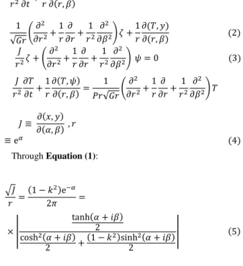
𝑥𝑥 + 𝑖𝑖𝑖𝑖 = − _2𝜋𝜋 ¹ ln �1 + (1 − 𝑘𝑘 ² ) tanh ^{2 𝛼𝛼+𝑖𝑖𝑖𝑖} ₂ � (1)

−∞ < 𝛼𝛼 ≤ 0, −|𝛽𝛽| ≤ 𝜋𝜋, −0 < 𝑘𝑘 < 1

where (x, y) is a dimensionless Cartesian coordinate system with vertically upward y. In this system, the reference length, L, is given by the distance between two parallel plates, i.e., the upper and lower plates are given by 𝑖𝑖 = 0.5 and 𝑖𝑖 = −0.5 respectively. It is assumed that the point ( 𝛼𝛼, 𝛽𝛽) = (0, 0) corresponds to point O, and (𝛼𝛼, 𝛽𝛽) = (0, 𝜋𝜋/2) to point A.

Consequently, the upper plate is designated by 𝛼𝛼 = 0, 2 tan ⁻¹ (1/√1 − 𝑘𝑘 ² ) < 𝛽𝛽 < 𝜋𝜋, the lower plate by 𝛼𝛼 = 0,

−𝜋𝜋 < 𝛽𝛽 < −2 tan ⁻¹ (1/√1 − 𝑘𝑘 ² ) and the fin by 𝛼𝛼 = 0,

−𝜋𝜋/2 ≤ 𝛽𝛽 ≤ 𝜋𝜋/2. The centerline AB (or A’B’) corresponds to 𝛼𝛼 = 0, 𝜋𝜋/2 < |𝛽𝛽| < 2 tan ⁻¹ (1/√1 − 𝑘𝑘 ² ). The system of governing equations for substantially incompressible Newtonian fluids under a Boussinesq approximation consists of the equation of vorticity transport, the relationship between vorticity 𝜁𝜁 and stream function 𝜓𝜓, and energy equation:

𝐽𝐽 𝑟𝑟 ²

𝜕𝜕𝜁𝜁

∂𝑡𝑡 + 1 𝑟𝑟

∂(𝜁𝜁, 𝜓𝜓)

∂(𝑟𝑟, 𝛽𝛽) = 1

√𝐺𝐺𝑟𝑟 � ∂ ²

∂𝑟𝑟 ² + 1 𝑟𝑟

∂

∂𝑟𝑟 + 1 𝑟𝑟 ²

∂ ²

𝜕𝜕𝛽𝛽 ² � 𝜁𝜁 + 1 𝑟𝑟

∂(𝑇𝑇, 𝑖𝑖)

∂(𝑟𝑟, 𝛽𝛽) (2) 𝐽𝐽

𝑟𝑟 ² 𝜁𝜁 + � ∂ ²

∂𝑟𝑟 ² + 1 𝑟𝑟

∂

∂𝑟𝑟 + 1 𝑟𝑟 ²

∂ ²

𝜕𝜕𝛽𝛽 ² � 𝜓𝜓 = 0 (3) 𝐽𝐽

𝑟𝑟 ²

∂𝑇𝑇

∂𝑡𝑡 + 1 𝑟𝑟

∂(𝑇𝑇, 𝜓𝜓)

∂(𝑟𝑟, 𝛽𝛽) = 1 𝑃𝑃𝑟𝑟√𝐺𝐺𝑟𝑟 � ∂ ²

∂𝑟𝑟 ² + 1 𝑟𝑟

∂

∂𝑟𝑟 + 1 𝑟𝑟 ²

∂ ²

𝜕𝜕𝛽𝛽 ² � 𝑇𝑇

𝐽𝐽 ≡ ∂(𝑥𝑥, 𝑖𝑖)

∂(𝛼𝛼, 𝛽𝛽) , 𝑟𝑟

≡ e ^𝛼𝛼 (4) Through Equation (1):

�𝐽𝐽 𝑟𝑟 =

(1 − 𝑘𝑘 ² )e ^−𝛼𝛼

2𝜋𝜋 =

× �

tanh(𝛼𝛼 + 𝑖𝑖𝛽𝛽) cosh ² (𝛼𝛼 + 𝑖𝑖𝛽𝛽) 2

2 + (1 − 𝑘𝑘 ² )sinh ² (𝛼𝛼 + 𝑖𝑖𝛽𝛽) 2

� (5)

2.2 Physical boundary conditions

The following fully Dirichlet type thermal boundary

conditions (not producing stratification) are introduced: along

the lower plate T = 0, along the left part of upper plate (DE) T

413

Journal of the Korean Society of Marine Engineering, Vol. 40, No. 5, 2016. 6

= 0, and along the right part of upper plate (CD) T =1, and along the fin (both sides) T = T C (0 < T C < 1). As a dynamical boundary condition, no-slip flows on the plates and on the fin surfaces are assumed ; i.e., without loss of generality, 𝜓𝜓 = 0 along the upper and lower plates, 𝜓𝜓 = c (constant to be determined) along the fin surface, and ^∂𝜓𝜓

∂𝛼𝛼 = 0 along the plates and the fin surfaces.

2.3 Mathematical boundary conditions Mathematical boundary conditions along 𝜶𝜶 = 0, 𝝅𝝅/2 < |𝜷𝜷| <

2 𝐭𝐭𝐭𝐭𝐭𝐭 ^−𝟏𝟏 (𝟏𝟏/√𝟏𝟏 − 𝒌𝒌 ^𝟐𝟐 )

Under Equation (1), the continuity of scalar quantity ϕ(α, β) at the both sides of center line (AB, A’B’) and the continuity of gradient vector for the scalar quantity ϕ(α, β) are given by

𝜙𝜙(0, 𝛽𝛽) = 𝜙𝜙(0, −𝛽𝛽) (6) 𝜕𝜕

𝜕𝜕𝛼𝛼 𝜙𝜙 (0, 𝛽𝛽)

= − 𝜕𝜕

𝜕𝜕𝛼𝛼 𝜙𝜙 (0, −𝛽𝛽) , (7)

which applies for 𝜓𝜓, 𝜁𝜁, and T.

2.4 Mathematical boundary conditions at r = 0( 𝛂𝛂 = -∞) At the single point given by r = 0, any scalar quantity and its gradient are independent of β, which is a necessary condition.

2.5 Conditions of doubly-connectedness

The condition for the region of doubly-connectedness is given by

� 𝜕𝜕𝜕𝜕

𝑓𝑓 𝜕𝜕𝛽𝛽 𝑑𝑑𝛽𝛽 = 0 (8) where p stands for pressure and f for integration around the fin.

Equation (8) leads to

1

√𝐺𝐺𝑟𝑟 � 𝜕𝜕𝜁𝜁

𝑓𝑓 𝜕𝜕𝛼𝛼 𝑑𝑑𝛽𝛽 + � 𝑇𝑇 𝜕𝜕𝑖𝑖

𝑓𝑓 𝜕𝜕𝛽𝛽 𝑑𝑑𝛽𝛽 = 0 (9) Under the given thermal boundary condition, Equation (9) becomes

� 𝜕𝜕𝜁𝜁

𝑓𝑓 𝜕𝜕𝛼𝛼 𝑑𝑑𝛽𝛽 = 0 (10)

2.6 Spectral decomposition of the unknowns

Among many possibilities of complete sets, Fourier series expansion is applied; that is:

� 𝜓𝜓(𝑟𝑟, 𝛽𝛽, 𝑡𝑡) 𝜁𝜁(𝑟𝑟, 𝛽𝛽, 𝑡𝑡)

𝑇𝑇(𝑟𝑟, 𝛽𝛽, 𝑡𝑡) � = � � 𝜓𝜓 _{𝑠𝑠𝑠𝑠} (𝑟𝑟, 𝑡𝑡) 𝜁𝜁 𝑠𝑠𝑠𝑠 (𝑟𝑟, 𝑡𝑡) 𝑇𝑇 𝑠𝑠𝑠𝑠 (𝑟𝑟, 𝑡𝑡) �

∞ 𝑠𝑠=1

𝑠𝑠𝑖𝑖𝑠𝑠 𝑠𝑠𝛽𝛽

+ � � 𝜓𝜓 𝑐𝑐𝑠𝑠 (𝑟𝑟, 𝑡𝑡) 𝜁𝜁 _{𝑐𝑐𝑠𝑠} (𝑟𝑟, 𝑡𝑡) 𝑇𝑇 _{𝑐𝑐𝑠𝑠} (𝑟𝑟, 𝑡𝑡) �

∞ 𝑠𝑠=0

𝑐𝑐𝑐𝑐𝑠𝑠 𝑠𝑠𝛽𝛽 (11)

The mathematical boundary conditions (6) and (7) for the arguments in Equation (11) become

𝜓𝜓(1, 𝛽𝛽, 𝑡𝑡) + 𝜓𝜓(1, −𝛽𝛽, 𝑡𝑡)

= 𝜁𝜁(1, 𝛽𝛽, 𝑡𝑡) + 𝜁𝜁(1, −𝛽𝛽, 𝑡𝑡) = 𝑇𝑇(1, 𝛽𝛽, 𝑡𝑡) + 𝑇𝑇(1, −𝛽𝛽, 𝑡𝑡) = 0 (12)

𝜕𝜕

𝜕𝜕𝑟𝑟 {𝜓𝜓(1, 𝛽𝛽, 𝑡𝑡)} + {𝜓𝜓(1, −𝛽𝛽, 𝑡𝑡)}

= 𝜕𝜕

𝜕𝜕𝑟𝑟 {𝜁𝜁(1, 𝛽𝛽, 𝑡𝑡)} + {𝜁𝜁(1, −𝛽𝛽, 𝑡𝑡)}

= 𝜕𝜕

𝜕𝜕𝑟𝑟 {𝑇𝑇(1, 𝛽𝛽, 𝑡𝑡)} + {𝑇𝑇(1, −𝛽𝛽, 𝑡𝑡)} = 0 (13) if 𝜋𝜋/2 < |𝛽𝛽| < 2 tan ⁻¹ (1/√1 − 𝑘𝑘 ² ). Equations (12) and (13) mean that the odd components of 𝜓𝜓, 𝜁𝜁 and T at r = 1 become 0 in the described interval, and that the derivative (with respect to r) for the even components of 𝜓𝜓, 𝜁𝜁 and T at r = 1 also become 0 in the described interval. Thus, the mixed boundary conditions at r = 1 can be split into Fourier components in the similar way as references in [1] and [8]. The boundary condition at r = 0 is given as a necessary condition.

𝜓𝜓 _{𝑠𝑠𝑠𝑠} (0, 𝑡𝑡) = 𝜁𝜁 𝑠𝑠𝑠𝑠 (0, 𝑡𝑡) = 𝑇𝑇 𝑠𝑠𝑠𝑠 (0, 𝑡𝑡) = 0 (𝑠𝑠 ≥ 1) (14) 𝜓𝜓 _{𝑐𝑐𝑠𝑠} (0, 𝑡𝑡) = 𝜁𝜁 𝑐𝑐𝑠𝑠 (0, 𝑡𝑡) = 𝑇𝑇 𝑐𝑐𝑠𝑠 (0, 𝑡𝑡) = 0 (𝑠𝑠 ≥ 1) (15) 𝜕𝜕

𝜕𝜕𝑟𝑟 𝜓𝜓 ^𝑐𝑐0 (0, 𝑡𝑡) = 𝜕𝜕

𝜕𝜕𝑟𝑟 𝜁𝜁 ^𝑐𝑐0 (0, 𝑡𝑡) = 𝜕𝜕

𝜕𝜕𝑟𝑟 𝑇𝑇 ^𝑐𝑐0 (0, 𝑡𝑡) = 0 (16) The constant c (to be determined) can be included in Equation (10), noting that J = 0 if α = β = 0.

2.7 Numerical integration of the governing Equations

The system of Equations (2) - (4) can be split into each

Fourier component, supplemented with the decomposed

boundary conditions at r = 1 and r = 0. Spatial and time

derivatives can be replaced by finite difference approximation

(nonuniform grid spacing can be accepted), which can be semi-

implicitly integrated with respect to time, using a suitably

given initial thermal and fluid flow field to get a steady-state

solution. Since the temperature on the fin surface is uniform,

414

Journal of the Korean Society of Marine Engineering, Vol. 40, No. 5, 2016. 6 the total dimensionless force F (based on 𝜌𝜌𝑈𝑈 ² 𝐿𝐿 , 𝑈𝑈 ≡

√𝐺𝐺𝑟𝑟 𝜈𝜈/L, 𝜈𝜈 ; kinematic viscosity) acting on the fin (z ≡ x + iy) becomes

−𝑭𝑭 = 𝑖𝑖

√𝐺𝐺𝑟𝑟 � 𝑧𝑧 ^′

𝑓𝑓 𝜁𝜁𝑑𝑑𝛽𝛽 − 𝑖𝑖

√𝐺𝐺𝑟𝑟 � 𝑧𝑧

𝑓𝑓

𝜕𝜕𝜁𝜁

𝜕𝜕𝛼𝛼 𝑑𝑑𝛽𝛽 (17)

The mean Nusselt number on the fin surface, N 𝑢𝑢 𝑚𝑚 , is given by

𝑁𝑁𝑢𝑢 𝑚𝑚 = ∮ _𝑓𝑓 ^{𝜕𝜕𝜕𝜕} _{𝜕𝜕𝛼𝛼} 𝑑𝑑𝛽𝛽 ∮ �𝐽𝐽 � _𝑓𝑓 𝑑𝑑𝛽𝛽 (18)

In this problem, the Dirichlet thermal boundary condition is assumed. Thus if N 𝑢𝑢 _𝑚𝑚 > 0 is positive, the heat is emitted outward from the fin as a heat source, and if N 𝑢𝑢 _𝑚𝑚 < 0 is negative, the heat is absorbed inward to the fin, as a heat sink.

Consequently, at −∞ < 𝛼𝛼 ≤ 0, if ^∂𝜕𝜕 _∂α > 0, the heat flux is outward and if ^∂𝜕𝜕 _∂α < 0, the heat flux is inward.

3. Numerical results and discussion

Figures 2 and 3 show streamlines and isotherms at √1 − 𝑘𝑘 ²

= 0.9, 𝑇𝑇 _𝑐𝑐 = 0.35, Gr = 10, and Pr = 0.7 (fin width = 0.264) respectively, where the characteristic values are N 𝑢𝑢 𝑚𝑚 = 0.32, F = 0.070i, and c = −0.0075. c < 0 presents clockwise circulation. For not a sufficiently large Grashof number, Gr, the characteristic values are nearly insensitive to Pr. Figures 4 and 5 show streamlines and isotherm at √1 − k ² = 0.8, T c = 0.35, Gr = 10, and Pr = 0.7 (fin width = 0.163) respectively, where the characteristic values are N 𝑢𝑢 _𝑚𝑚 = 0.49, F = 0.398i, and c =

−0.028. Figure 6 shows isotherms at √1 − k ² = 0.9, 𝑇𝑇 𝑐𝑐 = 0.15, Gr = 10, and Pr = 0.7, where the characteristic value are N 𝑢𝑢 𝑚𝑚 = −0.52, F = 0.039i, and c = −0.043.

Figure 2 : Streamlines at √1 − k ² = 0.9, T c = 0.35, Gr = 10, Pr = 0.7 and δψ = −0.001

Figure 3 : Isotherms at √1 − k ² = 0.9, 𝑇𝑇 𝑐𝑐 = 0.35, Gr = 10 and Pr = 0.7

Figure 4 : Streamlines at √1 − k ² = 0.8, 𝑇𝑇 𝑐𝑐 = 0.35, Gr = 10, Pr = 0.7 and 𝛿𝛿𝜓𝜓 = −0.005

Figure 5 : Isotherms at √1 − k ² = 0.8, 𝑇𝑇 𝑐𝑐 = 0.35, Gr = 10 and Pr = 0.7

Figure 6 : Isotherms at √1 − 𝑘𝑘 ² = 0.9, 𝑇𝑇 _𝑐𝑐 = 0.15, Gr = 10 and Pr = 0.7

415

Journal of the Korean Society of Marine Engineering, Vol. 40, No. 5, 2016. 6 Undisturbed (without any fin) pure conduction temperature

distribution is given by

𝑇𝑇 = � 1

(2𝑠𝑠 + 1)𝜋𝜋 e ^{(2𝑠𝑠+1)𝛼𝛼}

∗

∞ 𝑠𝑠=0

× sin(2𝑠𝑠 + 1) 𝛽𝛽 ^∗

− � 1

(2𝑠𝑠 + 1)𝜋𝜋 e ^{(4𝑠𝑠+2)𝛼𝛼}

∗

∞ 𝑠𝑠=0

× sin(4𝑠𝑠 + 2) 𝛽𝛽 ^∗

− � (−1) ^𝑠𝑠

(2𝑠𝑠 + 1)𝜋𝜋 e ^{(2𝑠𝑠+1)𝛼𝛼}

∗

∞ 𝑠𝑠=0

× cos(2𝑠𝑠 + 1) 𝛽𝛽 ^∗ + 1

4 (19)

𝛼𝛼 ^∗ + 𝑖𝑖𝛽𝛽 ^∗ ≡ ln �tan �𝑖𝑖 𝜋𝜋

2 (𝑥𝑥 + 𝑖𝑖𝑖𝑖)�� (20)

which shows that T c at O is 0.25. Thus, as long as √1 − k ² is not very near unity, the fin would behave as a heat source if T c > 0.25, and as a heat sink if T c < 0.25, which is coincident with Figures 3 and 6.

4. Conclusions

Natural convention heat transfer from a two-dimensional fin in the parallel enclosure was successfully analyzed, using a spectral finite difference scheme, supplemented with a condition of doubly-connectedness of the domain. The enclosure plates were placed horizontally and kept at constant temperatures. Problems were treated as a boundary-value problem, and variables were exactly decomposed into Fourier components. To get a steady-state solution, a time-marching scheme was applied. Depending on the uniform surface temperature of fin, the fin behaved as a heat source or sink.

References

[1] Y. Mochimaru, “Effectiveness of a spectral finite difference scheme,” Computational Fluid Dynamics Review, vol. 1, pp. 379-394, 1998.

[2] L. I. Volkovyskii, G. I. Lints, and I. G. Aramanovich, “A collection of problems on complex analysis,” Pergamon Press, 1965.

[3] P. Henrici, Applied and Computational Complex Analysis, vol. 1, Wiley, 1974.

[4] L. N. Trefethen, Numerical Conformal Mapping, North- Holland, 1986.

[5] R. Schinzinger and P. A. A. Laure, Conformal Mapping, Elsevier, 1991.

[6] Y. Mochimaru, “Existence/non-existence of conformal mapping in some family of functions,” International Journal of Pure and Applied Mathematics, vol. 49, pp.

497-503, 2008.

[7] Y. Mochimaru, “Analytical treatment of far away field behavior,” Computational Fluid Dynamics Journal, vol. 13, pp. 422-426, 2004.

[8] Y. Mochimaru, “Extension of applicability of a spectral finite difference scheme to mixed boundary conditions,”

Transport Phenomena in Thermal-Fluids Engineering, pp.

315-320, 1996.

[9] I. Catton (Ed. Kankaç, Aung, Vskanta), Natural Convection in Horizontally Unbounded Plane Layers, Natural Convection, Fundamentals and Applications, Hemisphere Pub, pp. 97-134, 1985.

[10] F. A. Kulacki and D. E. Richards (Ed. Kankaç, Aung, Vskanta), Natural Convection in Plane Layers and Cavities with Volumetric Energy Sources, Natural Convection, Fundamentals and Applications, Hemisphere Pub, pp. 179-255, 1985.

[11] R. Viskanta (Ed. Kankaç, Aung, Vskanta), Natural Convection in Melting and Solidification, Natural Convection, Fundamentals and Applications, Hemisphere Pub, pp. 845-877, 1985.

[12] P. G. Simpkins and K. S. Chen (Ed. Kankaç, Aung, Vskanta), Natural Convection in Horizontal Containers with Applications to Crystal Growth, Natural Convection, Fundamentals and Applications, Hemisphere Pub, pp.

1010-1032, 1985.

[13] A. G. Bathelt and R. Viskanta, “Heat transfer and interface motion during melting and solidification around a finned heat source/sink,” Transactions of ASME, Journal of Heat transfer, vol. 3, pp. 720-726, 1981.

[14] Y. Mochimaru, “A spectral finite difference scheme and its effectiveness,” Proceedings of 26th Annual Iranian Mathematics Conference, pp. 245-254, 1995.

[15] Y. Mochimaru, “Global instability of natural convection in an elliptic cavity, Using a fourier spectral difference method,” 7th Int. Coll. on Differential Equations, pp. 243- 252, 1997.

416

Journal of the Korean Society of Marine Engineering, Vol. 40, No. 5, 2016. 6 [16] D. Akita and Y. Mochimaru, “Numerical simulation of a

flow past an elliptic cylinder at moderately high reynolds numbers,” CMMPG, vol. 1, pp. 1-7, 2015.

[17] Y. Mochimaru and M. W. Bae, “A study on natural convection from two cylinders in a cavity,” Journal of Mechanical Science and Technology, vol. 20, no. 10, pp.

1773-1778, 2006.

[18] Y. Mochimaru and M. W. Bae, “Natural convection heat transfer in a doubly - connected region, using a spectral

finite difference scheme,” International Journal of Pure and Applied Mathematics, vol. 32, no. 1, pp. 51-60, 2006.

[19] Y. Mochimaru and M. W. Bae, “Spectral analysis on natural convection heat transfer from a rectangular cylinder partially heated in an infinite extension (Invited Lecture),” International Journal of Pure and Applied Mathematics, vol. 46, no. 2, pp. 237-243, 2008.

417