실험데이터처리 Data mining
Ch. 1 Introduction
Major: Interdisciplinary program of the integrated biotechnology
Graduate school of bio- & information technology Youngil Lim (N110), Lab. FACS
Youngil Lim (N110), Lab. FACS
phone: +82 31 670 5200 (secretary), +82 31 670 5207 (direct) phone: +82 31 670 5200 (secretary), +82 31 670 5207 (direct)
Fax: +82 31 670 5209, mobile phone: +82 10 7665 5207 Fax: +82 31 670 5209, mobile phone: +82 10 7665 5207 Email:
Email: [email protected][email protected], homepage:, homepage: http://facs.maru.nethttp://facs.maru.net
Course # Course name Time Room #
Data mining Thu. 9-12 시 N130/N116
Overview
In recent year, there has been stunning progress in data mining and machine learning. The synthesis of statistics, machine learning, information theory and computing has created a solid science, with a firm mathematical base, and with very powerful tools. This lecture presents the basic theory of automatically extracting models from experimental data, and then validating those models. This lecture includes a multivariate linear regression, training/testing/validation techniques, principle component analysis (PCA), partial least square (PLS) and artificial neural network (ANN) algorithms. Matlab or Weka toolkit is used for computational practices. This lecture is given in English.
Method Lecture(●), Seminar (●), Computational practice (●), Factory tour (●), Beam projector(●)
Evaluation Attendance: 8%, homework: 20%, Mid-exam: 30%, Final-exam: 30%, Presentation: 12%
Text
Main : Witten and Frank, Data mining: practical machine learning tools and techniques, Elsevier, 2005.
Outline
Week Contents Remarks 1 Introduction
2 EndNote 13, Uses and practices Presentation 1: EndNote
3 Part I. Machine learning tools and techniques, Ch. 1 what is it all about?
4 Part I. Machine learning tools and techniques, Ch. 2 input data 5 Part I. Machine learning tools and techniques, Ch. 3 output data
6 Field trip (Factory tour, October 7, 2010) KITECH, Biomass gasifier (Dr. Lee Uen-Do) 7 Part I. Machine learning tools and techniques, Ch. 4 algorithms Presentation 2: ch. 4
8 Part I. Machine learning tools and techniques, Ch. 4 algorithms 9 Mid-term exam.
10 Part II. The weka program, Ch. 9 Introduction to Weka
11 Part II. The weka program, Ch. 10 Explorer of Weka ? 12 Field trip (Factory tour):
13 Part II. The weka program, Ch. 10 Explorer of Weka
14 Ammonia emission problem (Lim et al., 2007) Analysis of Lim et al. (2007) 15 Final exam. (Report on the ammonia emission problem)
Weekly Lecture Plan
Overview of this lecture
- Machine learning = acquisition of structural descriptions automatically or semi-auto.
(it is similar as the brain development from repeating experiences) - Weka written in JAVA (object-oriented programming language)
(JAVA is free to OS and its calculation is 2-3 times slower than C, C++ and Fortran - Java compiler (Java virtual machine) translate the byte-code into machine code
Information (data, database)
Knowledge
(understanding, application, prediction)
Data mining
(extraction of useful information)
input (ch. 2)
output (ch. 3)
Relationships?
Modeling
Structural patterns
Technical tools: machine learning
Outline of this lecture
Part I. Machine learning tools and techniques
- Level 1: Ch 1. Applications, common problems
Ch 2. Input, concepts, instances and attributes Ch 3. Output, knowledge representation
- Level 2: Ch 4. Numerical algorithms, the basic methods - Level 3: Ch 5-6 (advanced topics)
Part II. Weka manual (ftp://facs/lim/lecture_related/weka3.4.exe) - Level 1: Ch 9. Introduction of Weka
Ch 10. Explorer
- Level 2: Ch 11-15 (advanced options in Weka)
But, you need to read those chapters to make a paper on data mining
Ch. 1. What’s it all about
Human in vitro fertilization
60 embryos fertilized select just 1 embryo What is the decision criteria?
Life and death
It is up to Machine Learning
inputs (attributes) - morphology - oocyte
- …
outputs (results) Live or die
Cow breeding of farmers
- 1/5 cows to be abated - 4/5 cows to be bred
What is the decision criteria?
inputs (attributes) - age
- health - calving - …
outputs (results) Live or die
- Data mining: process of discovering structural patterns in data.
- Machine learning: technical tools for finding structural patterns in data automatically or semi-automatically.
1.1 data mining and machine learning
- See Table 1.1
- there are 4 attributes (descriptors) - there are 3 decisions (outputs)
- 24 possibilities and 24 instances - no data missing
- no noise in data
- perfect prediction is possible - It is an ideal and fictitious example
Describing structural patterns
- learning and training
- training = mindless learning - Machine learning includes
numerical algorithms for automatic calculations
Machine learning
1.1 data mining and machine learning
Table 1.1
- Different datasets tend to expose new issues, challenges, and different numerical algorithms (case by case).
1.2 sample examples: weather problems and others
- See Table 1.2
- there are 4 attributes (descriptors) - there are 2 decisions (outputs)
- 36 possibilities and 14 instances - decision list in order (see p11) - numeric-attribute problem
- mixed-attribute problem
- The classification rule is one of the association rules, and it is the best rule.
1. The weather problem
- machine learning is to
- identify the data structure - predict for new cases
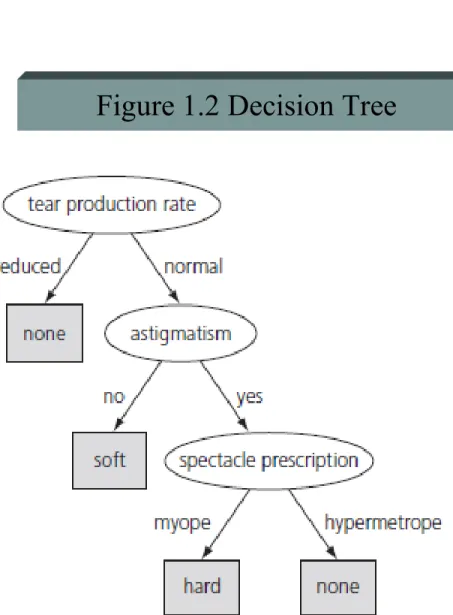
- see Table 1.1, Figure 1.1, and Figure 1.2
- which representation is better
understandable between Figure 1.1 and Figure 1.2?
2. Contact lenses: ideal case
In Ch. 3,
We will learn more classification/association rules
1.2 Examples
Table 1.2
Table 1.3
Figure 1.1
Figure 1.2 Decision Tree
1.2 Examples
1.2 sample examples: weather problems and others
- See Table 1.4 (Fisher, 1935) - there are 4 attributes
- numeric-attribute problem - see p16.
- Output is the 3 categories
- More compact rule is in Ch. 3.
That is we use the following statement:
if … then …
else if … then … end if
3. Irises: numerical dataset
- see Table 1.5
- there are 6 attributes
- Output is estimated by multi-variable linear regression (MLR)
- prediction of numeric performance
- Numerical algorithms will be reviewed in ch. 4
4. CPU performance: numeric prediction
1.2 examples
Table 1.4
1.2 examples
Table 1.5
1.2 sample examples: weather problems and others
- see Table 1.6
- there are 16 attributes and 40 examples - missing data but realistic case
- 2 decisions (acceptable or not) - see Figure 1.3 (a) and (b)
- (a) simple and intuitive decision tree
- (b) complex and accurate representation - which is the artifact and overfited?
- Ch. 5 and 6 concern about cross- validation and missing data
5. Labor negotiation
- see Table 1.7
- a successful story of ML techniques - soybean disease diagnosing
- 35 attributes and 680 examples - 19 outputs (categories)
- 97.5% accuracy over 72% of expert - the expert adopted ML rules
6. Soybean classification
1.2 examples
Table 1.6
1.2 examples
Table 1.7
1.3 Fielded applications
- for borderline applicants of loan (sub-prime loan) - there are about 20 attributes
- there are 2 decisions (accept or not) - the borrowers pay off or default
- correct predictions from ML are related to the profit of the loan company.
1. Decision of loan company
- For warning ecological disasters
- oil slicks appear as dark regions in the image - the detection is an expensive manual process - this problem is challenged because
- scarcity of training data
- a very small fraction are actual oil slicks - batch process (case by case)
2. Screening satellite images for oil slicks detection
The previous examples are speculative and toy problems.
Where is the beef?
1.3 Fielded applications
- for estimating Max. and Min. of load for hour, day, month, season, and year - there are many attributes (day/night, holiday, weekend, weather …)
- we need a dynamic model
- ML system is far quicker than the trained human forecasters.
- a few seconds or a few days
3. Power load forecasting in electricity supply industry
- For determination of the kind of fault,
- the diagnosis process is too labor intensive - 1000 different devices, and noisy data
- outputs are 600 faults
- low level attributes from vibration records of devices - derived attributes from Fourier’s analysis
- ML performance is slightly superior to that of expert 4. Diagnosis of machines and devices
1.3 Fielded applications
- for planning store layouts, special discounts, offering coupons, … - attributes: costumer’s purchase records (by membership card)
market basket analysis - econometrics
- detecting customers who is fickle and defect 5. Marketing and sales
- control problems of plants
- biology: identification of genes
- biomedicine: prediction of drug activity, and 3D structure - astronomy:
- chemistry: structure identification of certain organic compounds - automation
6. Other applications
1.4 Machine learning and statistics
What is the difference between ML and statistics?
- ML: statistics + marketing
- Statistics: ML that has arisen out of computer science - But, two perspectives have converged
- Statistical tests are used to validate ML models and to
evaluate ML algorithms
1.6 data mining and ethics
Data mining is used for people, it provokes ethical
problems such as racial, sexual and religious
1.5 Generalization as search
ML and statistics = generalization as search
This section is optional, as indicated by the gray bar !
Field trip report
(as a scientific report)
Components or contents
1. Introduction: backgrounds, states-of-art, aims, and short overview of the report
2. Main body: Knowledge or information from field trips, applications, results, and analyses 3. Conclusion: summary, and perspectives
4. Reference: books, papers, patents, reports, websites
5. Appendix: accessory information
An example of field trip report
Application of data mining to a process in Petro-chemical company, Samsung Total Miso Kim ([email protected]), 200720111
Dept. Chemical engineering, Hankyong National University Gyonggi-do Anseong Jungangno 167, 456-749 Korea
1. Introduction
1.1 What is data mining?
1.2 Aims of this report 1.3 Overview of this report
2. Main processes of Petro-chemical plant of Samsung Total.
2.1 PE and PP processes 2.2 BTX processes 2.3 …
* Each table and each figure have own number and title. Those tables and figures should be well explained in the text.
3. Application of data mining tools 3.1 PE (poly ethylene) process 3.2 Expected attributes
3.3 Main objectives of machine learning technique in the PE process 4. Conclusions
Appendix
A1. Rector flowsheet of PE (poly-ethylene) process A2. …
References
Douglas, J. M. (1998), Conceptual design of chemical processes, McGraw-Hill, p124.
Lim, Y.-I, Son, H.-J. (2007), Multiscale simulation for adsorption process, Comput. Chem. Eng., 45, p234-459.