A time-cost tradeoff problem with multiple interim assessments under the precedence graph with two chains in parallel
1)Byung-Cheon Choi*, Yunhong Min**
Abstract
We consider a project scheduling problem in which the jobs can be compressed by using additional resource to meet the corresponding due dates, referred to as a time-cost tradeoff problem. The project consists of two independent subprojects of which precedence graph is a chain. The due dates of jobs constituting the project can be interpreted as the multiple assessments in the life of project.
The penalty cost occurs from the tardiness of the job, while it may be avoided through the compression of some jobs which requires an additional cost. The objective is to find the amount of compression that minimizes the total tardy penalty and compression costs. Firstly, we show that the problem can be decomposed into several subproblems whose number is bounded by the polynomial function in , where is the total number of jobs. Then, we prove that the problem can be solved in polynomial time by developing the efficient approach to obtain an optimal schedule for each subproblem.
▸Keyword: Project scheduling, Time-cost tradeoff, Parallel precedence graph
I. Introduction
In project management, a manager need to consider two conflicting objectives: (1) minimizing project completion time and (2) minimizing the project cost. The completion time, referred to as a makespan, of a project can be reduced by investing more resources which incurs the increase of project cost. The time-cost tradeoff problem (TCTP) has a form either of minimization of the project’s cost under a specified due date or of minimization of makespan under a given budget.
When the makespan of a project is considered either as an objective or a constraint, we assume that only one assessment exists during the whole project. In reality, however, there may exist multiple assessments in the middle of the project with respect to the corresponding interim due dates, and thus some penalties can occur if the project at each
assessment does not go along according to a planned schedule.
For example, a venture capital company begins to makes small investments on a start-up and then determines whether the additional investment is carried out or not, based on what the start-up achieves compared with its initial plan [3, 14].
In this paper, we consider the TCTP with multiple assessments in which a project consists of multiple jobs and some jobs have their own due dates. Jobs with their own due dates are called milestones. In general, there exist the precedence relations among jobs and these relations are represented by the graph, called the precedence graph. In the precedence graph, each node corresponds to job and the arc between two jobs represents their precedence.
∙First Author: Byung-Cheon Choi, Corresponding Author: Yunhong Min
*Byung-Cheon Choi ([email protected]), School of buisiness, Chungnam National University
**Yunhong Min ([email protected]), Graduate School of Logistics, Incheon National University
∙Received: 2018. 01. 30, Revised: 2018. 02. 05, Accepted: 2018. 02. 28.
∙This work was supported by research fund of Chungnam National University in 2017.
Each job has its own processing time which can be compressed through the use of some resources, e.g., human or capital. If a milestone fails to be completed within its due date, it incurs the penalty cost. The penalty cost, however, can be avoided by reducing or compressing the processing time of some jobs. The objective is to minimize the sum of the tardiness and the compression costs. We describe the tardy and compression costs as a weight of the tardy milestone and the linear function for the amount of compression, respectively.
Our project scheduling problem belongs to the class of the TCTP with the linear compression cost function, referred to as a LTCTP. For a comprehensive review of the TCTP with more general compression cost function (e.g., convex or concave), see [2, 10, 12, 13]. Fulkerson [9] and Kelley [11] considered the LTCTP to minimize the makespan, subject to a constraint on the budget for the total amount of compression, and proposed an efficient algorithm based on the network flow model. Choi and Chung [5] considered two LTCTP’s with multiple milestones on a single chain precedence graph. The objective of the first is to minimize the total weighted number of tardy jobs with a constraint on the total compression cost. The second objective is to minimize the sum of the total compression cost and the total weighted number of tardy jobs. They proved the weak NP-hardness of the first problem and the polynomiality of the second. Choi and Park [6] considered the general version of the second problem in [5] such that the compression cost function is convex or concave. They proved the weak NP-hardness and the polynomiality of the problems with the concave and the convex compression cost functions, respectively. Choi and Chung [7] considered the problem in [6] with the concave compression cost function, and investigated the optimality properties that make the problem polynomially solvable.
The problem in this paper can be considered as the general version of the problem in [5, 6, 7], in that more general precedence graph, i.e., two chains in parallel, is considered. The precedence graph of two chains in parallel is motivated from the situation such that
The project consists of several independent subproject whose precedence graph can be described as a chain.
The project is started after dividing up the project into several subproejcts, and completed after assembling the completed subprojects.
Our problem can be formally stated as follows. The problem can be represented by a activity-on-node graph
consisting of two chains in parallel, where
is the set of jobs and is the set of precedence relations. Then, the resulting precedence graph is described as Fig. 1. Let the jobs in
be referred to as the set of start and terminal jobs.
Fig. 1. The precedence graph
For the chain , is the set of jobs consisting the chain . Associated with job
∈, is an initial processing time , a maximal amount for compression and a compression cost ratio
. Let ∈ be the vector of which component is the compression amount of job subject to ≤ ≤ . Note that ∈
completely characterizes the schedule, because there exists an optimal schedule such that each job is started as soon as possible. Thus, we call ∈ a schedule. Let job be uncompressed and fully compressed in a schedule , if and , respectively. Let ⊆ be the set of milestones, i.e., jobs with due dates. For ∈, let and be the due date and the penalty cost for tardiness of milestone
, respectively. Let be the completion time of job in a schedule . Note that we can transform the case with ⊆ into the one with by letting
∈
and for ∈. It is clear that the optimal schedules of the original and transformed cases are identical. Without loss of generality, henceforth, we assume that , and call milestone as job. Our problem, called Problem P, can be formulated as follows:
min
∈
∈
′′ ′′≤′′ ′′ ∈
≤ ≤
where is the set of tardy jobs in . To exclude a trivial case, we assume that the zero vector with
for each ∈ is not an optimal schedule.
The remainders of the paper are organized as follows.
Section 2 decomposes Problem P into the smaller subproblems whose polynomialities imply the polynomiality of Problem P. Section 3 develops the effi cient algorithms for each subproblem. Finally, Section 4 presents some concluding remarks and future works.
II. Decomposition of Problem P
In this section, we show that Problem P can be decomposed into the subproblems by using the concept of the just-in-time (JIT) job. A job is said to be just-in-time (JIT), if it is completed exactly at in an optimal schedule. Firstly, we present some optimality conditions.
Lemma 1 There exists an optimal schedule such that at least one JIT job exists.
Proof. Suppose that a job is compressed and the JIT job does not exist in an optimal schedule . We can construct a new schedule by letting where
is sufficiently small value. Since and
∈
∈
however, . This is a contradiction. ■
Lemma 2 There exists an optimal schedule such that the jobs after the last JIT jobs in ∪ and ∪ are uncompressed.
Proof. If job (0,2) is the JIT job in an optimal schedule
. Then, we assume that job (0,2) is not the JIT job in
. Suppose that in there exists a compressed job
after the last JIT jobs in ∪or ∪. Then, we can construct a new schedule by letting where is sufficiently small value. Since
and
∈
∈
however, . This is a contradiction. ■
For each , let and be the first and
the last JIT jobs on chain in the optimal schedule, respectively. Depending on the existences of jobs and on each chain , the structure of the optimal schedule belongs to one of the three cases in Fig. 2. Note that if chain has one JIT job, then
for each .
In Case 1, both chains have the JIT job, while in Cases 2 and 3, either one and neither of chains has no JIT job, respectively.
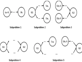
It is observed that if we know the existences and positions of JIT jobs in an optimal solution, the schedules of the remaining jobs in the optimal solution can be obtained by solving some of subproblems in Fig. 3. For example, Cases 1 and 2 consist of subproblems 1–3 and subproblems 1 and 5, respectively.
By the observation above, we can have the following theorem.
Theorem 1 Problem P can be solved in polynomial time if the five subproblems in Fig. 3 are polynomially solvable.
Proof. It is observed that the possible number of the cases is depending on which jobs in each chain become the first and the last JIT job. Since each case belongs to one type of Cases 1–3 and consists of at most four subproblems in Fig. 3, the total number of the subproblems that we should solve to find an optimal schedule for Problem P is . Henceforth, we show that Problem P is polynomially solvable by proving the polynomiality of Subproblems 1–5. ■
Fig. 2. Three cases
Fig. 3. Five subproblems
III. Polynomiality of Subproblems
In this section, we show that five subproblems in Fig. 3 are polynomially solvable. It is known from [5] that the polynomial solvability of Subproblem 1 was proved. Thus, we consider only Subproblems 2–5. The following notation is useful for the subsequent expositions. For each chain ,
and
1. Subproblem 2
For simplicity, we introduce some notation. For each chain , let
min min and max max,
where ∆
∈∪
and
arg for ∈ (1)
If multiple jobs have the minimum compression cost ratio in (1), then the one processed earliest is selected, because this way guarantees the schedule with the smallest total penalty for the tardy jobs.
Lemma 3 There exists an optimal schedule for Subproblem 2 such that
(i) If max min then,
min min for .
(ii) If max min and ≤
then, minmin.
(iii) If max min and
then,
≥ minmin
for .
Proof. Firstly, consider the case (i). Without loss of generality, assume that max and min. Suppose that
min . This implies the existence of job with
≤
and
. If
then we can construct a new schedule by letting
and
where is sufficiently small. Since , this is a contradiction. If
, then we can construct a new schedule by letting
and
where min
. Since job is processed before job , . By applying this argument repeatedly, we can construct another optimal schedule satisfying (i) or a contradiction occurs.
The cases (ii) and (iii) can be proved by the similar argument, and hence we omit them. ■
Based on Lemma 3, we can construct an algorithm to obtain an optimal schedule for Subproblem 2 as follows:
Algorithm Out-Tree
Step 1. Set and for and
.
Step 2. Find .
Step 3. If max min then go to Step 3-1, while go to Step 3-2, otherwise.
Step 3-1 For , update
and max by letting
,
,
and
max max max,
where min min, and go to Step 3-3 Step 3-2 If ≤
, then update and m in by letting
, , and min min ,
where minmin.
Otherwise, for , update
and min by letting
,
,
and min min,
where minmin
.
Step 3-3 If min , then STOP.
Step 3-4 If , then set ∞ and go to Step 2.
Note that Algorithm Out-Tree runs in .
Theorem 2 Subproblem 2 can be solved in polynomial time.
Proof. It holds immediately from Algorithm Out-Tree.
■
2. Subproblem 3
It is observed from Lemma 2 that if job (0,2) is not a JIT job, then all jobs are uncompressed in an optimal schedule for Subproblem 3. Thus, we assume that job (0,2) is a JIT job in the optimal schedule. For chain
, let
min and max max,
where max∈∪
and
arg for ∈ (2)
If multiple jobs have the minimum compression cost ratio in (2), then the one processed earliest is selected, because this way guarantees the schedule with the smallest total penalty. Then, we can characterize the properties of the optimal schedule of which statements and proofs are similar to Lemma 3 (Thus, we omit the proof).
Lemma 4 There exists an optimal schedule for Subproblem 3 such that
(i) If max min then,
min min for .
(ii) If max min and ≤
then, minmin.
(iii) If max min and
then,
≥ minmin
for .
Based on Lemma 4, we cam construct an algorithm to obtain an optimal schedule for Subproblem 3 as follows:
Algorithm In-Tree
Step 1. Set and for and
.
Step 2. Find .
Step 3. If max min then go to Step 3-1, while go to Step 3-2, otherwise.
Step 3-1 For , update
and max by letting
,
,
and max max max,
where min min, and go to Step 3-3.
Step 3-2 If ≤
, then update and min by letting
, , and min min ,
where minmin. Otherwise, for , update
and min by letting
,
,
and min min ,
where minmin
.
Step 3-3 If min , then STOP.
Step 3-4 If , then set ∞ and go to Step 2.
Note that Algorithm In-Tree runs in .
Theorem 3 Subproblem 3 can be solved in polynomial time.
Proof. It holds immediately from Algorithm In-Tree. ■
3. Subproblem 4
In this subsection, we show that Subproblem 4 can be reduced to either Subproblem 2 or Subproblem 3..
Lemma 5 There exists an optimal schedule for Subproblem 4 such that at least one of jobs in is fully compressed or uncompressed.
Proof. Suppose that each job in is partially compressed in . Consider two cases.
(i) ≠ : For simplicity, let . We can construct a new schedule by letting and
where is sufficiently small value.
Then, it is observed that
and
∈
∈
which implies .
(ii) : We can construct a new schedule by letting and , where
min . It is observed that
≤ and
∈
∈
which implies ≤ . ■
Theorem 4 Subproblem 4 can be solved in polynomial time.
Proof. By Lemma 5, it suffices to consider the following two cases
(i) Job (0,1) is fully compressed or uncompressed: In this case, Subproblem 4 is reduced to Subproblem 3 with new jobs (0,3) and (0,4) such that the processing times of jobs (0,3) and (0,4) are or , and their maximal amount for compressions are zeros (See Fig. 4).
Fig. 4. The precedence graph for Subproblem 3 reduced from Subproblem 4
(ii) Job (0,2) is fully compressed or uncompressed: If job (0,2) is not a JIT job, then it is observed from Lemma 2 that in an optimal schedule ,
for ∈∪∪.
Thus,
max i f max≤ and ≤
where . If job (0,2) is a JIT job, then Subproblem 4 is reduced to Subproblem 2 with new JIT jobs (0,5) and (0,6) such that the processing times of jobs (0,5) and (0,6) are or and their maximal amount for compressions are zeros (See Fig. 5). ■
Fig. 5. The precedence graph for Subproblem 2 reduced from Subproblem 4
4. Subproblem 5
For Subproblem 5, it is observed from Lemma 2 that if job (0,2) is not a JIT job, all jobs in ∪∪ are uncompressed in an optimal schedule, which implies that Subproblem 5 is reduced to Subproblem 1. Thus, to exclude this case, throughout this subsection we assume that job (0,2) is a JIT job.
Lemma 6 If at least one of jobs in is fully compressed or uncompressed in an optimal schedule, then Subproblem 5 is decomposed into some of Subproblems 1-3.
Proof. Consider two cases.
(i) Job (0,1) is fully compressed or uncompressed:
Subproblem 5 is reduced to Subproblems 1 and 3 with new jobs (0,3) and (0,4) such that the processing imes of jobs (0,3) and (0,4) are or , and their maximal amount for compressions are zeros (See Fig. 6).
Fig. 6. The precedence graphs for Subproblem 1 and 3 reduced from Subproblem 5
(ii) Job (0,2) is fully compressed or uncompressed:
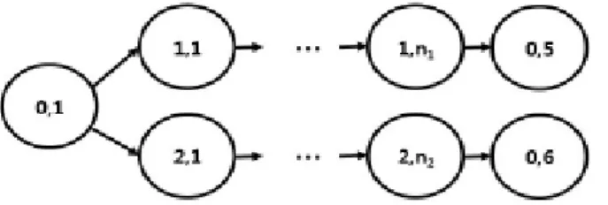
Subproblem 5 is reduced to Subproblems 1 and 2 with new JIT jobs (0,5) and (0,6) such that the processing times of jobs (0,5) and (0,6) are or , and their maximal amount for compressions are zeros (See Fig. 7) ■
Lemma 7 Suppose that jobs (0,1) and (0,2) are partially compressed in an optimal schedule . Then, there exists an optimal schedule for Subproblem 5 such that all jobs in or are fully compressed or uncompressed.
Fig. 7. The precedence graphs for Subproblems 1 and 2 reduced from Subproblem 5
Proof. Suppose that jobs ∈ and ∈ are partially compressed in . Consider two cases.
(i) ≠ : For simplicity, let
. Then, we can construct a new schedule by letting , ,
, and where is sufficiently small value. Then, it is observed that
and
∈
∈
which implies .
(ii) : We can construct a new schedule by letting , ,
, and where
min . It is observed that
≤ and
∈
∈
which implies ≤ . ■
Lemma 8 Suppose that jobs (0,1) and (0,2) are partially compressed in an optimal schedule . If a partially compressed job exists in for , then, Subproblem 5 is reduced to Subproblem 2, while it is reduced to Subproblem 3, otherwise.
Proof. Consider two cases.
(i) A partially compressed job exists in for : By Lemma 7, this case implies that the jobs in are fully compressed or uncompressed in . Let
max arg for ∈
and
min arg for ∈
Then, it is observed that ∈
becomes the one of the vectors such that
Some jobs are fully compressed and the others are uncompressed;
max≤
min; If
max
min, job max is processed before job
m in.
For example, assume that ≤ ≤
. Then, the set of these vectors is
Note that the value of corresponding to each vector can be determined because job (0,2) is a JIT job.
The precedence graph corresponding to each vector is the second graph in Fig. 7.
(ii) A partially compressed job exists in for : By Lemma 7, this case implies that the jobs in are fully compressed or uncompressed in . Thus this case is similarly proved by changing the role of and in e case (i). The precedence graph corresponding to this case is the second graph in Fig. 6. ■
Theorem 5 Subproblem 5 can be solved in polynomial time.
Proof. It holds immediately from Theorems 2-3 and Lemmas 6-8. ■
IV. Conclusions
We consider the LTCTP with the multiple interim assessments, when the precedence graph is two chains in parallel. The objective is to minimize the total weighted number of tardy jobs plus the total compression cost.
Firstly, we decompose the problem into subproblems, based on JIT jobs whose number is bounded by the total number of jobs. Then, we show that our problem is polynomially solvable by proving the polynomiality of each subproblem.
For future research, it would be interesting to consider the case such that the precedence graph consists of more than two chains in parallel, or the compression cost function is convex or concave function.
REFERENCES
[1] C. Artigues, D. Demassey., E. Neron. “Resource- Constrained Project Scheduling,” Wiley, 2008.
[2] E.B. Berman. “Resource allocation in a PERT network under continuous activity time–cost function,”
Management Science Vol. 10, pp. 734–745, July 1964.
[3] J. Bell. “Beauty is in the eye of the beholder: Establishing a fair and equitable value for embryonic high-tech enterprises,” Venture Capital Journal, Vol. 40, pp. 33–34,
Jan. 2000.
[4] P. Bruker, A. Drexl, R. Mohring, K. Neumann, and E.
Perch. “Resource-constrained project scheduling:
Notations, classfication, models and methods,” European Journal of Operational Research, Vol. 112, pp. 3–41, Jan.
1999.
[5] B.C. Choi, and J.B. Chung. “Complexity results for linear time-cost tradeoff problem with multiple milestones and completely ordered jobs,” European Journal of Operational Research, Vol. 236, pp. 61–68, July 2014.
[6] B.C. Choi, and M.J. Park. “A continuous time-cost tradeoff problem with multiple milestones and completely ordered jobs,” European Journal of Operational Research Vol. 244, pp. 748–752, Aug. 2015.
[7] B.C. Choi, and J.B. Chung. “Some special cases of a continuous time–cost tradeoff problem with multiple milestones under a chain precedence graph,”
Management Science and Financial Engineering, Vol. 22, pp. 5–12, May 2016.
[8] E.L. Demeulemeester and W.S. Herroelen. “Project scheduling - A research handbook,” Kluwer Academic, 2002.
[9] D.R. Fulkerson. “A network flow computation for project cost curves,” Management Science, Vol. 7, pp. 167–178, Jan. 1961.
[10] J.E. Falk, and J.L. Horowitz. “Critical path problems with concave cost–time curves,” Management Science, Vol.
19, pp. 446–455, Dec. 1972.
[11] J.E. Kelley. “Critical path planning and scheduling:
Mathematical basis,” Operations Research, Vol. 9, pp.
296–320, June 1961.
[12] L.R. Lamberson, and R.R. Hocking. “Optimum time compression in project scheduling,” Management Science, Vol. 16, pp. 597–606, June 1970.
[13] J. Moussourakis, and C. Haksever. “Project compression with nonlinear cost functions,” Journal of Construction Engineering and Management, Vol. 136, pp. 251–[259, Feb. 2010.
[14] W.A. Sahlmann. “Insights from the ventures capital model of project governance,” Business Economics, Vol. 29, pp. 35–41, July 1994.
[15] J. Weglarz. “Project scheduling - Recent models algorithms and applications,”Kluwer Academic, 1999.
[16] J. Weglarz, J. Jozefowska, M. Mika, and G. Waligora.
“Project scheduling with finite or infinite number of activity processing modes - a survey,” European Journal of Operational Research, Vol. 208, pp. 177–205, Feb.
2011.
Authors
Byung-Cheon Choi received the B.S. and Ph.D. in Industrial Engineering from Seoul National University in 2000 and 2006, respectively. Dr. Choi joined the faculty of School of Business at Chungnam National University in 2009. He is currently an professor in School of Business at Chungnam National University. He is interested in combinatorial optimization, scheduling theory, and operations management.
Yunhong Min received the B.S. degree in Industrial Engineering & Management Science from POSTECH, and Ph.D. in Industrial Engineering from Seoul National University in 2006 and 2012, respectively.
Dr. Min joined the faculty of Graduate School of Logistics at Incheon National University in 2017.
Before joining Incheon National University, he was a research staff member of Samsung Advanced Institute of Technology. He is interested in mathematical optimization and machine learning and their applications to logistics and supply chain management.