Vol. 12, No. 2, p. 123−137, June 2008 DOI 10.1007/s12303-008-0014-9
Modeling of water flow and heat transport in the vadose zone: Numerical demonstration of variability of local groundwater recharge in response to monsoon rainfall in Korea
ABSTRACT: The rainfall of Korea in the summer monsoon period occupies more than 50% of the annual precipitation in most areas, and thus groundwater recharge to shallow aquifers is dominantly controlled by the amount and the pattern of monsoon precipita- tion. This paper presents two numerical models that demonstrate linear relationships between precipitation and recharge. First, a simple heat transport model employing a lumped parameter approach is presented for estimating two lumped parameters related to water flux and thermal diffusivity in the vadose zone.
The model determines the parameters by a simple optimization process that minimizes the root-mean-square error between sim- ulated and measured temperatures. The model is applied to 22- year time series data of soil temperatures measured at a synoptic station of Korea. The impact of monsoon precipitation on the ther- mal regime is clearly reflected in the simulated results by illus- trating a linear relationship between precipitation and the water flux in the vadose zone. Secondly, an infiltration model is pre- sented for analyzing variability of precipitation recharge in rela- tion to the monsoon rainfall. The model simulates the unsaturated flow from time series data of precipitation and pan evaporation, assuming immediate removal of surface ponding, a linear rela- tionship between the evaporation rate and the soil water content, and a static water table. Numerical simulations were performed for three soil textural groups by using 20-year meteorological data.
The results demonstrate that the annual recharge is linearly pro- portional to the annual precipitation with varying degrees of the correlation coefficient depending on soil types. Sensitivity analyses show that the uncertainties in evaporation-related model param- eters significantly affect the model results with controlling tradeoff between recharge and evaporation estimates.
Key words: groundwater recharge, monsoon, vadose zone, heat transport model, infiltration model, finite difference method, Korea 1. INTRODUCTION
The subsurface temperature has long been used as a tracer for indirect measurement of water movement based on the hypothesis that heat in the subsurface is transported by con- duction as well as advection caused by subsurface water movement. Due to wide potential uses of subsurface tem- perature data, numerous methodologies ranging from simple analytical methods to complex coupled models have been
investigated in a variety of hydrogeological settings. A com- prehensive review of recent work can be found in Anderson (2005). One of the earlier attempts utilizing subsurface tem- perature as a tracer was made by Stallman (1965) who pre- sented an analytical solution for computing infiltration rates from transient temperatures observed near the land surface.
The solution was based on the assumption of a sinusoidal temperature fluctuation at the land surface and a constant and uniform percolation rate normal to the land surface in a homogeneous medium. Later this method was employed and expanded in many studies such as evaluation of vertical groundwater fluxes (Taniguchi, 1993), groundwater-surface water interactions (Silliman et al., 1995), and determination of groundwater recharge (Taniguchi and Sharma, 1993; Tab- bagh et al., 1999). However, the analytical methods have inher- ent limitations in applications, since they require a steady periodicity assumption for boundary conditions and temper- ature measurements over long annual cycles. Recently the temperature methods to quantify water movement in the subsurface have been expanded to use of numerical models (Ronan et al., 1998; Constantz et al., 2002; Constantz et al., 2003) that do not require the assumption of a steady peri- odicity and can be applied for shorter time period.
Since the early 1990s, a number of infiltration models have been introduced in the literature to describe infiltration and the subsequent recharge process from the vadose zone to the groundwater system. Hendrickx et al. (1991) used a tran- sient finite difference model and a steady-state analytical solution to evaluate the travel time of the recharge water and the maximum annual recharge volume. Based on a numer- ical model simulating soil-water movement, Wu et al. (1996) analyzed the effect of rainfall patterns and annual rainfall distribution on infiltration recharge at different groundwater depths. Wu et al. (1997) used a response function model to estimate soil water flux at the water table and the process of infiltration recharge from rainfall and evaporation data. Pohll et al. (1996) simulated the movement of water during seep- age beneath a nuclear subsidence feature by using a coupled surface-subsurface hydrologic model, which can compute the movement of surface water, the mass balance of the pon- Min-Ho Koo
Yongje Kim* Department of Geoenvironmental Sciences, Kongju National University, Kongju, Chungnam 314-701, Korea Groundwater and Geothermal Research Division, Korea Institute of Geoscience and Mineral Resources (KIGAM), Daejeon 305-350, Korea
*Corresponding author: [email protected]
ded water, the subsequent infiltration, and the vertical mois- ture movement. Binley et al. (1997) demonstrated the role of model parameter uncertainty on estimates of recharge by means of Monte Carlo simulations. Recently, attempts to deal with both hydrological and ecological parameters (Zhang et al., 1999a; Zhang et al., 1999b; Guswa et al., 2002) and to analyze multi-dimensional rainfall infiltration (Disse, 1999; Zhou et al., 2002) were made to provide a more real- istic description of the infiltration process in the vadose zone.
Korea has unique meteorological characteristics influ- enced by the summer monsoon which starts in the southern region of Korea in late June (Fig. 1) and gradually proceeds northward. Ho and Kang (1988) investigated spatial and temporal variation of precipitation in Korea using the rain- fall data during the 23-year period of 1963-1985. The mean annual precipitation of Korea is 1,287 mm/yr. The rainfall in the summer monsoon period occupies more than 50 % of the annual precipitation in most areas, and the intensity of the rainfall frequently exceeds 100 mm/day. These meteorolog- ical features suggest that the amount of annual groundwater recharge is dominantly controlled by the amount and the pat- tern of rainfall occurring during the monsoon season. Thus, the monsoon should be a critical hydrologic component determining the groundwater recharge. Due to temporal variability of precipitation, which is very high especially in the monsoon region, vertical water movement in the vadose zone is also a time variant process and thus the approaches or models should account for transient behaviors of thermal properties and water fluxes.
In this paper, two numerical models, a heat transport model and an infiltration model, are presented to examine how variability of monsoon precipitation would impact the groundwater recharge in Korea. The heat transport model, solving the inverse problem by using time series temperature data, is aimed to reveal seasonal variations of water fluxes and thermal properties in the vadose zone in response to monsoon precipitation. The model can eliminate limitations of analytical models and can expand the potentiality of sub- surface temperature technique in real field situations. The infiltration model is also developed to simulate the recharge process using time series data of precipitation and pan evap- oration. It simulates flow features in the vadose zone includ-
ing infiltration, surface ponding, evaporation and groundwater recharge. The developed model is used to analyze variability of precipitation recharge for various soil types in response to the monsoon rainfall in Korea.
2. HEAT TRANSPORT MODEL FOR ESTIMATING PERCOLATION RATES
2.1. Model Development
Temperature at the land surface is controlled principally by an energy balance between incoming solar radiation and outgoing long wavelength thermal radiation. Changes in the land surface temperature with time occur at several temporal scales. The largest of these changes are the daily and sea- sonal variations, both of which can have amplitudes of 10 degrees or more. Temperature below the surface is affected by the flux of heat being conducted below from the land surface as well as the heat flux conducted out from the earth’s interior and the heat transfers resulting from other external or internal physical, chemical and biological pro- cesses. The subsurface medium acts as a low-pass filter and attenuates these thermal waves with depth. The high fre- quency or short term variations die out more rapidly than long term variations.
The advective heat transfer resulting from water move- ment is also a major process that controls the subsurface temperature within the vadose zone mostly encountered in real situations. When precipitation occurs on the land sur- face, a part of the precipitation infiltrates down through the vadose zone as a source of groundwater recharge and the heat is also transported below the land surface as mass trans- fer. Thus, the movement of water results in the transfer of heat through the advective process as well, which leads to the redistribution of heat within the subsurface and altering the subsurface temperature distribution. Relative importance of these mechanisms in controlling the subsurface thermal regime is site specific and may vary in space and time.
2.1.1. Heat transport equation
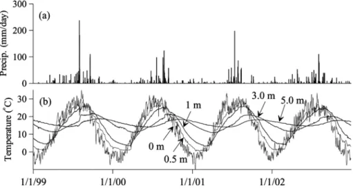
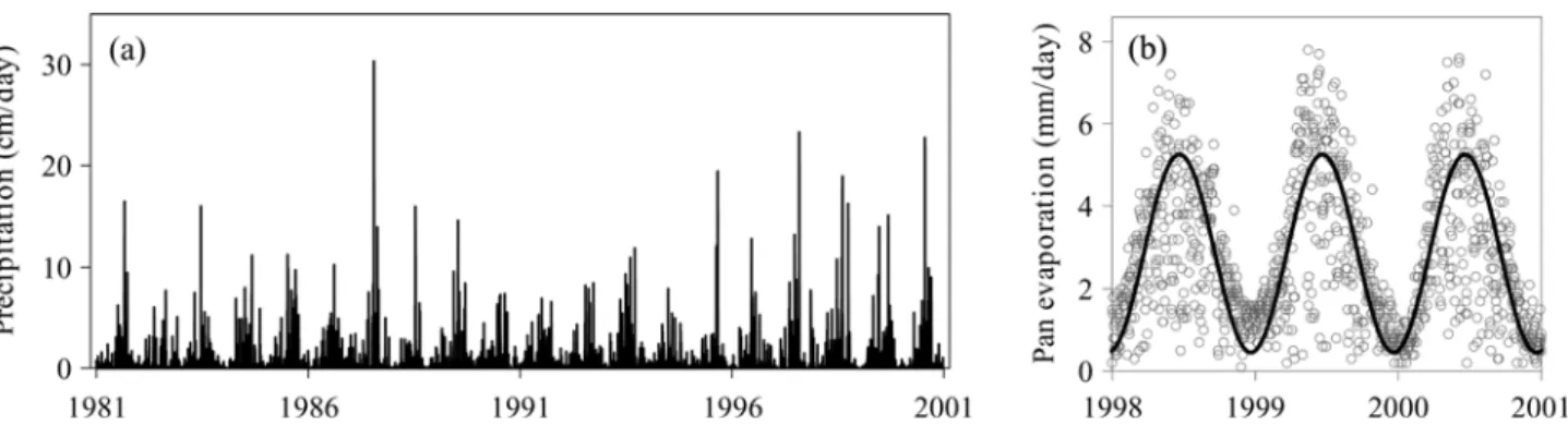
The one-dimensional governing equation for the conduc- tive and advective transport of heat through the vadose zone Fig. 1. Temporal variation of precipi- tation in Korea: (a) daily precipitation averaged over the period of 1971-2000 and (b) annual precipitation measured at the Daejeon synoptic station.
can be expressed as (Healy and Ronan, 1996):
(1) where T is temperature, t is time, z is the depth from the ground surface taken as positive downward, q is volumetric water content, φ is porosity, Cw and Cs are volumetric heat capacity (density times specific heat) of water and the dry solid, respectively, KT is thermal conductivity of the bulk medium, Dh is the thermomechanical dispersion coefficient, and qw is vertical water flux. The bracket in the left side of the equation represents the volumetric heat capacity of the bulk medium, where the heat capacity of air is ignored.
It is evident from Eq. (1) that the solution requires time- dependent specification of q and qw which leads to a coupled system of heat and water flow. Furthermore, additional information on the relationship between KT and q should be known, since KT strongly varies with q. Therefore, the heat transport in the vadose zone is a complicated nonlinear process coupled with water flow, and it should be sequentially solved with the unsaturated flow within an iterative framework as in VS2DH (Healy and Ronan, 1996). Although solving the coupled process of heat and water flow can provide a more precise description of the heat transport process in the vadose zone, it is less practical in applications to the inverse problem due to the extensive uncertain input parameters and computational requirements. As discussed in the second part of this paper, the unsaturated flow model also requires numerous input parameters. Although Ronan et al. (1998) attempted to use VS2DH for estimating streambed infiltration rates from subsurface temperature data, many of the model parameters for the simulations were based on representative values reported in the literature. Thus, it is extremely unlikely that incorporating all the parameters with an acceptable level of accuracy into the coupled model could be practically possible.
Therefore, due to difficulties in data availability of the coupled model, a simplification of Eq. (1) is employed in this study by assuming that the model parameters are uni- form in space and time-independent during a certain period of time. The simplified equation can be expressed as:
(2) where α and β are lumped parameters to be estimated in the inverse process given by:
(3)
(4)
The conductive and dispersive components of heat transport in Eq. (1) are combined into the first term in the right side of Eq. (2). Thus, a can be viewed as ‘apparent’ or ‘effective’
thermal diffusivity which is analogous to the hydrodynamic dispersion coefficient in the advection-dispersion equation for solute transport. β is the parameter that includes the rate of vertical water flow. Thus, complex processes associated with heat transport in the vadose zone are simplified by nullifying temporal variations of thermal and hydraulic parameters. Validation of this assumption can be achieved by selecting an appropriate period of time depending on temporal variability of precipitation that determines the water content and flow in the shallow vadose zone.
2.1.2. Finite difference method
The MacCormack scheme is used to solve Eq. (2) with appropriate initial and boundary conditions. This scheme is based on the second-order forward-time Taylor series:
(5) where i is the space index, n is the time index, Δt is time interval, and subscript t with variable T indicates its time derivative. In the MacCormack scheme, is determined directly from the partial differential equation (PDE) and is determined from a second-order forward-time Taylor series expansion for :
= (6)
Combining Eq. (5) and Eq. (6) yields:
= (7)
Eq. (7) can be solved by dropping the truncation error terms and replacing and in terms of spatial derivatives from the PDE:
(8)
The MacCormack scheme utilizes a two-step predictor- corrector approach to evaluate explicitly for the considered heat transport equation. In the first step, and are approximated by the first-order forward difference approximation. The resulting finite difference equation of the first step for the PDE given by Eq. (2) can be expressed as:
(9) where CN and DN are cell convection number and cell dif- fusion number, respectively. These numbers are expressed as:
∂t∂
----[θCw+(1–φ)]T ∂
∂z--- KT∂T ---∂z
⎝ ⎠
⎛ ⎞ ∂
∂z--- θCwDh∂T ---∂z
⎝ ⎠
⎛ ⎞
+
=
∂z∂
---(CwqwT) –
∂T∂t
--- α∂2T
∂z2 --- β∂T
---∂z –
=
α KT( )θ θCw+(1–φ)Cs
--- θCwDh
θCw+(1–φ)Cs
--- +
=
β Cwqw
θCw+(1–φ)Cs
---
=
Tin 1+
Tin
TtniΔt 1
2---TttniΔt2+O Δt( 3)
+ +
=
Tt in
Ttt in Tt in 1+
Ttt in 1+ Ttni+TttniΔt +O Δt( 2)
Ttt in 1+ Tin 1
2---[Ttni+Ttn 1i+ ]Δt O Δt( 3)
+ +
Tt in Tt in 1+
Tin 1+
Tin 1
2---[αTzz in–βTz in+αTzz in 1+ +βTz in 1+ ]Δt +
=
Tin 1+
Tt in Tz in
Ttn 1+
Tin
CN Ti 1n+
Tin
( – )
– DN Ti 1n+
2Tin
– Ti 1n–
( + )
+
=
(10)
(11)
Results obtained from the first step (predictor) are the provisional values and are modified in the second step known as corrector step to get the final results. In the second step, Eq. (8) is solved by evaluating using the first-order forward difference approximation and using the first- order back ward difference approximation based on the provisional values of . Thus, the resulting equation for the second step can be written as:
(12) Eq. (9) combined with Eq. (12) comprises the MacCormack scheme approximation of Eq. (2) and can be solved with appropriate initial and boundary conditions of the system specific to the considered study area. The scheme is conditionally stable and convergent. The grid size and time scale for the considered application are chosen such that the cell convection and diffusion numbers are within the limits of CN ≤ 0.9 and DN ≤ 0.5 as reported by Hoffman (1992) for the MacCormack scheme to get the stable and convergent solutions.
2.1.3. Development of an inverse model
Based on the MacCormack finite difference solution of the simplified heat transport equation, an inverse model is developed to estimate the lumped parameters, α and β from the subsurface temperature measurements. The key to this inverse model is to optimize the model results by searching for the unknown parameters by using temperature data. The model requires temperature time series data measured at
three different depths. Two temperature data sets measured at the shallower and deeper depths are used as the upper and lower boundary conditions, and the temperature measured in the middle is used for optimization. Applications of the model also require an appropriate selection of depth and time intervals which meet the stability and convergence criteria discussed above. A simple sequential search is employed for the optimization process. A series of heat transport simulations are consecutively repeated by varying the unknown parameters within a possible range of each parameter. The performance of each simulation is evaluated by the root-mean-square error (RMSE) between simulated and measured temperatures, and optimization of the model is realized by searching for the values α and β which minimize RMSE.
2.2. Materials
2.2.1. Temperature data
The developed model is applied to ground temperature data measured at the Chuncheon synoptic station (37°54'N, 127°44'E) of the Korea Meteorological Administration (KMA).
The depths of temperature measurements are 0, 0.05, 0.1, 0.2, 0.3, 0.5, 1.0, 1.5, 3.0 and 5.0 m below the ground surface. The temperature data measured from 1981 to 2002 are used for the analysis. A process of quality control for raw data was conducted to eliminate some unacceptable temperatures which were thought to be associated with wrong readings or inputs by mistake. The elimination was performed by a simple numerical scheme where the temperature under inspection is regarded as a bad data, if it is higher or lower than the temperature of the previous day by more than 15 °C.
Figure 2 shows temporal variation of daily precipitation and ground temperatures at various depths measured at the Chuncheon station. A clear illustration of the amplitude decay and the phase delay is observed, indicating that con- duction is the dominant mechanism of heat transport in the shallow ground. The mean and the standard deviation of annual precipitation during the simulation period are 1290
CN βΔt
Δz---
=
DN α Δt
Δz ( )2 ---
=
Tz in Tz in 1+ Tn 1+
Tin 1+ 1 2--- Tin
Tin 1+
CNTin 1+
Ti 1n 1–+
– –
[ +
=
+DN Ti 1n 1++
2Tin 1+
– +Ti 1n 1–+
( )]
Fig. 2. Time series data of (a) daily precipitation and (b) soil temperature at various depths measured at the Chuncheon synoptic station of KMA.
mm/yr and 330 mm, respectively. Comparing these to the statistical values during the period of 1963-1985 given by Ho and Kang (1988) indicates that temporal variability of precipitation has been enhanced by 200 mm in the standard deviation for the last 20 years. Increase of the variability is mainly caused by the amount of rainfall in the summer mon- soon months.
2.2.2. Data partitioning
As mentioned above, the developed model assumes the lumped parameters which are constant with respect to time and space. Two alternatives can be taken into consideration in dealing with this simplifying condition. The first is to con- sider the lumped parameters to vary at every time interval of the measurements, so that they can be determined for each time step in simulations. This approach forces the model to determine the unknown parameters which make a perfect agreement between the measured and simulated tempera- tures and thereby it appears to be an attractive method of choice. However, as analyzed by Zang and Osterkamp (1995), this approach does not yield a reliable estimation of the unknown parameters, since it is vulnerable to large trun- cation errors during the period when the rate of temperature change becomes small and also it is highly sensitive to the effects of measurement errors. The second alternative assumes the unknown parameters to be constant within a certain period of time during which many temperature measure- ments are made, so that they can be determined by the least squares method as described above.
This study employed the second approach in the inverse model, and thus the model required a preprocessing for partitioning the temperature data into multiple segments that could attain approximate validation of the simplifying assumption. The data partitioning is based on the consideration that the temporal variation of the lumped parameters in the near surface is primarily controlled by precipitation, and also Korea is under the monsoon meteorological environments.
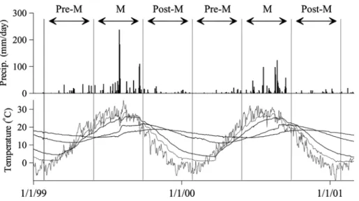
Based on the amount of precipitation, the 22-year temperature data is divided into 66 segments which consecutively correspond to a series of pre-monsoon, monsoon, and post-monsoon periods (Fig. 3). The model parameters α and β are assumed to be constant during the period of each segment, and they are estimated by the optimization procedure.
2.3. Simulation results
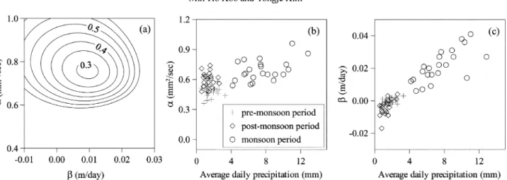
The model used the temperature data at 1 m and 5 m depth as upper and lower boundary conditions, respectively, and used the temperature at 3 m for optimization. The optimal values of α and β are searched for each data segment by minimizing the RMSE between simulated and measured temperatures at 3 m depth. Figure 4a shows how the RMSE for a time segment changes with varying both α and β. It is obvious from the figure that there are optimal values of α and β with which the RMSE attains its minimum, and the sensitivity of the model performance is similar for both α and β. It is also found that the model performance varies for different data segments, and it is generally more sensitive to changes in α, indicating that the diffusive heat transport which lumps the conductive and dispersive process as in Eq. (3) prevails over the advective transport in the associated depth interval.
The simulation results in Figure 4 clearly illustrate variability of the estimated parameters in response to monsoon precip- itation. Figure 4b reflects the cyclic variation of α, the effective thermal diffusivity, which is related to the variation of water content in the vadose zone. In the monsoon period, increase of the water content due to a great amount of precipitation causes an increase of the thermal conductivity as well as the dispersion coefficient of the vadose zone, resulting in the associated increase in the effective thermal diffusivity. The water content is lowered in the following post-monsoon period, and further more in the pre-monsoon period, which is demonstrated in Figure 4b. The correlation
Fig. 3. Partitioning of time series tem- perature data into multiple segments based on precipitation.
coefficient between α and the amount of precipitation is 0.63. Scattering found in the post-monsoon period can be attributed to variation of the water content at the end of the monsoon period, although not analyzed explicitly.
A similar cyclic variation is also observed in the estimates of β, the lumped parameter for water flux (Fig. 4c). During the monsoon period, a linear relationship between precipi- tation and β, having the correlation coefficient of 0.93, is clearly demonstrated in the simulation results. It is expected that the linearity would be also retained for the relationship between precipitation and the annual groundwater recharge, since the estimated percolation rate in the vadose zone represents the potential amount of recharge. During the pre- and post-monsoon periods, negative values of water flux are observed in the simulation results. It is likely that, if the net amount is considered, the persistent and upward water flux driven by evaporation in the near surface would exceed the sporadic and downward water flux by precipitation in the dry period. As could be observed in Figure 4c, this is more pronounced in the post-monsoon period in which the vadose zone holds much moisture for evaporation replenished during the monsoon period. On the contrary, the water flux almost ceases during the pre-monsoon period, since the
divergent zero flux plane, which has been progressively moved downward during the post-monsoon period lingers due to little evaporation, and the amount of precipitation is not enough to entirely sweep the upper zone of the zero flux plane.
The hydrothermal processes occurring in the near surface was also examined by using the temperature data measured at the depths of 0, 0.5, and 1 m. The results, although not given in this paper, showed considerable scatter in relation- ships between precipitation and the estimated parameters.
The most likely possibility is that other heat transfer mech- anisms would occur actively in the near surface, and thereby could cause a temperature variation to deviate from the the- oretical one based on the conductive and advective heat transport. As would be expected, soils near the surface in Korea are highly vulnerable to freezing and thawing. Figure 5 shows a clear evidence of the nonconductive heat transfer, illustrating variation of the ground temperature affected by latent heat associated with freezing and thawing of the near surface. During the months of the year when freezing and thawing of the ground surface occur (January – March), the ground temperature at a depth of 0.5 m is immune to change being affected by the latent heat released or absorbed during Fig. 4. Simulation results: (a) sensitivity of the RMSE over a range of two known parameters, (b) annual variations of α and (c) variations of β in response to precipitation.
Fig. 5. The effect of latent heat asso- ciated with freezing and thawing of the near surface observed in the tempera- ture data of the Chuncheon KMA sta- tion.
phase changes. Thus, the effect of latent heat in the cold sea- son highly disturbs the conductive temperature variation observed in other seasons. The persistence of a constant tem- perature close to zero degree is directly related to soil water content. It is intuitive that soils with higher water contents would undergo the latent heat effect for longer period of time. Soils with smaller particles generally have higher water contents due to their higher field capacity and lower permeability. Thus, it is probable that the latent heat effect would be more pronounced in fine-grained soils. In addition to the latent heat effect, freezing and thawing of soils also can affect the process of conductive heat transfer by con- trasting thermal diffusivities of water (0.14 mm2/sec) and ice (1.2 mm2/sec). The heat transport in soils near the surface is a very complicated process, being affected by the presence of water and its phase changes.
Although many researchers have used the subsurface tem- perature to quantify the rate of water fluxes in the subsurface (Taniguchi and Sharma, 1993; Silliman et al., 1995; Tabbagh et al., 1999), no attempt was made to analyze seasonal vari- ations of water fluxes. In spite of the simplifying assump- tions, the lumped parameter model presented in this paper could delineate seasonal variations of the hydrothermal pro- cess occurring in the vadose zone. However, the model can lead to erroneous predictions depending on the degree of discrepancies between the assumed and the real field situa- tions. It appears that availability of the model may be limited particularly for soils near the surface in Korea. The limited availability would be mainly associated with the freezing and thawing process as evidenced in Figure 5 as well as the convective heat transfer of air which is not directly accounted for in this paper.
3. INFILTRATION MODEL FOR ESTIMATING PRECIPITATION RECHARGE
3.1. Model development
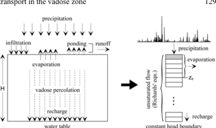
Figure 6 shows the conceptual model for the flow process of precipitated water occurring in the surface and the sub- surface of a bare soil. A transient finite difference model is developed to deal with the flow process by taking into account infiltration and surface ponding of precipitation at the top of the soil profile, evaporation, and the unsaturated flow in the vadose zone governed by Richards’ equation.
3.1.1. Richards’ equation
The vertical movement of soil water in the vadose zone is commonly described by Richards’ equation (RE). RE can be expressed by three different forms depending on selection of the dependent variable: the h-based, the θ-based, and the mixed forms. Recently, the mixed form has been widely used in finite difference or finite element methods, since it produces a perfect mass balance in the solution and simul-
taneously preserves advantages of the h-based form (Celia et al., 1990; Miller et al., 1998). A mixed form of RE can be expressed as
(13) where θ is the volumetric water content, h is the pressure head, K(h) is the unsaturated hydraulic conductivity, z is the positive downward, and r is the source/sink term by which evaporation and precipitation can be taken into account. In the developed model, the mass-conserving modified Picard iteration scheme of Celia et al. (1990) is used to solve the finite difference equation of RE.
In order to solve RE, the constitutive equations, which relate the pressure head to the moisture content and the rel- ative hydraulic conductivity, are required. The closed-form analytical expressions of van Genuchten (1980) are employed in the model:
(14)
(15) Where m = 1-1/n, Se is the effective saturation, θs and θr
are the saturated and the residual volumetric water contents, respectively, α and n are the fitting parameters related to soil properties, and Ks is the water-saturated hydraulic conduc- tivity.
3.1.2. Precipitation and surface ponding
It is assumed in the model that precipitation is not inter- cepted by the vegetation canopy, and gross precipitation reaches the soil surface. Thus, the time series data of pre- cipitation are imposed on the top layer of the finite differ- ence grid as source terms. When the top layer is saturated and the precipitation rate exceeds the infiltration rate during the monsoon period, precipitation begins to accumulate in the surface. In the model, the ponded water on the surface is assumed to be immediately removed by runoff. When the sur- face ponding occurs, the model automatically converts the
∂θ∂t --- ∂
∂z--- K h( )∂h
---∂z–K h( ) +r
=
Se θ θ– r
θs–θr
--- (1+ αhn)–m
= =
K= Ks Se[1–(1 S– e1 m⁄ )m]2
Fig. 6. Schematic diagram of the developed infiltration model.
pressure head of the top layer to zero. The amount of the pon- ded water is calculated by the mass balance of the top layer.
3.1.3. Evaporation
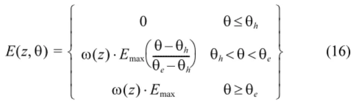
To evaluate the interdependence of the evaporation rate and the volumetric water content, the following relationships modified from the formulation of Guswa et al. (2002) are used to describe evaporation processes in the vadose zone:
(16)
where E is the evaporation rate per unit soil depth [1/T], ω is the depth-dependent weighting parameter [1/L], Emax is the maximum evaporation rate [L/T], θh is the volumetric water content at which evaporation ceases, and θe is the threshold water content at which evaporation reaches its maximum.
Evaporation is assumed to takes place over a depth ze, and the following exponential function is used to describe the weighting parameter:
(17)
(18) where λ is the parameter which determines the vertical dis- tribution of ω from the surface to a depth ze and ω0 is the weighting parameter at the soil surface. Combining Eqs.
(17) and (18) yields
(19)
Emax, the evaporation rate that would occur when the water content exceeds the threshold water content, is assumed to be the same as the pan evaporation rate measured at the sur- face synoptic station. Vapor flow driven by either pressure or temperature gradients in the vadose zone is ignored in the model, although it can be an important component in the water balance of the model, especially near the soil surface.
However, Hendrickx and Walker (1997) demonstrated that vapor flow could almost always be ignored for the assess-
ment of recharge rates in deep vadose zones where capillary rise from the aquifer could be neglected.
3.1.4. Source/sink term
Precipitation and evaporation are incorporated into the source/sink term of Eq. (13). Precipitation data are given into the source term of the top layer having the grid size of Δz, and evaporation as a sink term is calculated over the evaporation depth ze as given by Eq. (16). Thus, the source/
sink term in Eq. (13) can be expressed as
(20)
where p(t) is the precipitation rate [L/T]. Since E, the evap- oration rate per unit soil depth, is a function of the water content as given in Eq. (16), it is updated at every iteration step until convergence of the solution is achieved.
3.1.5. Boundary and initial conditions
The upper boundary condition is specified as no flow at the soil surface, and the lower boundary is considered as the water table which is assumed not to fluctuate with time. The initial conditions of the model are generated by running a certain period of preliminary cyclic simulation prior to the time of interest until the resulting solutions produce the same cyclic pattern. Preliminary simulations are performed by a multiple-year precipitation sequence having a cyclic pattern of the first-year precipitation sequence. Usually a 5-year of preparatory simulation is needed to produce the same cyclic pattern in this study. A more detailed explanation on the dynamic cyclic initial conditions can be found in Anderson and Woussner (1992).
3.2. Simulation results 3.2.1. Input data
Simulations are conducted for 3 soil textural groups: sand, loam and silt. Table 1 presents the van Genuchten parame- ters of the soils as estimated by Carsel and Parrish (1988) from analyses of a large number of soils. Table 1 also gives the model parameters used in the simulations. It is assumed that evaporation ceases at the effective saturation of 0.01 and evaporation reaches its maximum at the effective saturation E z θ( , )
0 θ θ≤ h
ω z( ) E⋅ max θ θ– h
θe–θh
---
⎝ ⎠
⎛ ⎞ θh< <θ θe
ω z( ) E⋅ max θ θ≥ e
⎩ ⎭
⎪ ⎪
⎪ ⎪
⎨ ⎬
⎪ ⎪
⎪ ⎪
⎧ ⎫
=
ω z( ) ω0 1 e– –λ z(e–z) 1 e– –λze ---
⋅ 0 z z( ≤ ≤ e)
=
ω zd
0 ze
∫ = 1
ω0 λ 1 e( – –λze) λze–(1 e– –λze) ---
=
r t z( ),
p t( )
--- E t z θΔz – ( , , ) 0 z Δz≤ ≤ E t z θ(, , )
– Δz z z< < e
0 z z≥ e
⎩ ⎭
⎪ ⎪
⎪ ⎪
⎨ ⎬
⎪ ⎪
⎪ ⎪
⎧ ⎫
=
Table 1. Selected van Genuchten parameters used in the study (Carsel and Parrish, 1988), and model parameters used in the simulations
Soil type θr θs α (cm-1) n Ks (cm/day) θh θe λ (cm-1) ze (cm) H (cm)
sand 0.045 0.43 0.145 2.68 712.8 0.049 0.122 0.001 30 500
loam 0.078 0.43 0.036 1.56 24.96 0.082 0.148 0.001 30 500
silt 0.034 0.46 0.016 1.37 6.00 0.038 0.119 0.001 30 500
of 0.2. The values of θh and θe in the table correspond to the effective saturation of 0.01 and 0.2, respectively. It is also assumed that evaporation takes place over a depth of 30 cm and the water table is at a depth of 500 cm. Twenty-year records (1981-2000) of daily precipitation and pan evapo- ration monitored at the Daejeon surface synoptic station (36°22'N, 127°22'E) of KMA are used as input data of the model simulations (Fig. 7). Figure 7b shows pan evaporation rates measured at the synoptic station during the period of 1998-2000. The solid line in the figure represents a least squares sinusoidal curve for the set of the measured data.
The best-fitting sinusoidal curve is used for temporal vari- ation of the maximum evaporation rate in Eq. (16).
3.2.2. Precipitation-recharge relationship
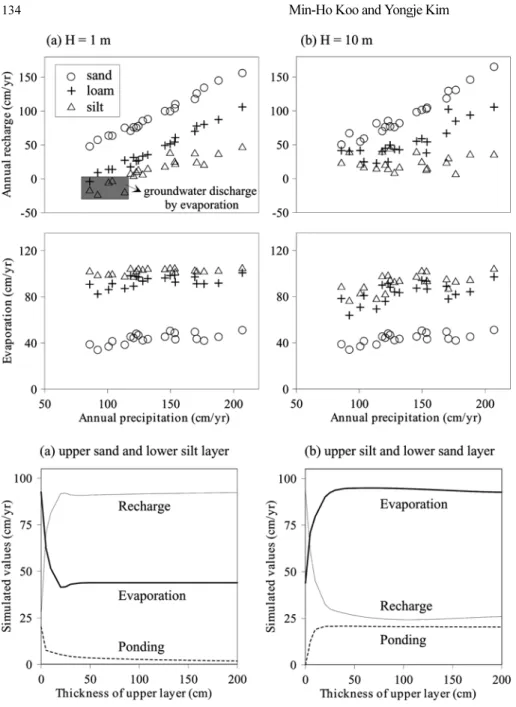
Shown in Figure 8 is the variations of annual recharge, evaporation, and surface ponding obtained from the 20-year transient simulations conducted with the input data dis- cussed above. Figure 8a clearly demonstrates that a linear relationship between annual precipitation and annual recharge holds with varying degrees of the correlation coefficient depending on soil types. Thus, the relationships can be expressed as
(21)
where, R is the annual recharge, P is the annual precipitation, P0 is the threshold precipitation below which no recharge takes place and μ is the ratio of recharge to the excessive precipitation (P-P0). Depending on the soil types, the esti- mated 20-year average annual recharge ranges from 265 mm/yr to 939 mm/yr which corresponds to 18% to 67% of the annual precipitation. A regression analysis of the simu- lated results shows that the threshold precipitation ranges from 350 mm/yr to 710 mm/yr, and the correlation coeffi- cient of the linear relations ranges from 0.65 to 0.98 showing a decreasing trend as the soil is getting finer.
Analyzing time series of the annual precipitation and the simulated annual recharge reveals that as the soil is getting finer, the annual recharge is more influenced by the precip- itation of the previous year. This indicates that variability of antecedent water content in the soil decreases the correlation coefficient of the linear relations especially for the finer soils. Deviation from the linearity is mainly caused by vari- ation of water storage in the vadose zone at the end of the former year. Thus, although not directly accounted for in the linear equation, the water content distribution of the soil prior to the year of interest should also be an important con- sideration in estimating annual recharge, particularly for fine-grained soils. Although the method using an empirical relationship between recharge and precipitation is criticized R=μ P P( – 0)
Fig. 7. Meteorological data measured at the Daejeon surface synoptic station: (a) daily precipitation and (b) pan evaporation (open circle) and the least squares sinusoidal curve (solid line).
Fig. 8. Simulated relationships between annual precipitation and (a) recharge, (b) evaporation, and (c) surface ponding for 3 different soil types.
in the literature (Gee and Hillel, 1988), the results show that it holds for the soils under the monsoon climates with vary- ing degrees of success depending on the soil types. Thus, as discussed by Allison et al. (1994), an empirical relationship between recharge and precipitation can be useful for making first-guess estimates of recharge in areas where annual recharge is fairly high. High variability of annual precipita- tion in the monsoon climates causes a wide range of annual recharge. The simulated annual recharge ranges from 57.2 to 78.7% of annual precipitation for the sand and 4.5 to 31.8%
for the silt. Thus, in order to evaluate recharge in terms of a fractional percentage of annual precipitation, recharge esti- mates should be averaged over several years.
Figure 8b shows the simulated relationships between annual precipitation and annual evaporation. Compared to the vari- ability of annual recharge to precipitation, evaporation is less influenced by the annual precipitation showing only a slight increase with increase of the annual precipitation. Figure 8c shows the simulated relationships between annual precipi- tation and surface ponding. No ponding occurs in the sand over the whole period of simulation due to its relatively high infiltration capability, while it occurs in the loam only in the years that have concentrated heavy rainfalls in the monsoon season. On the contrary, the amount of the ponded water in the silt is linearly proportional to precipitation. The linear relationship can be attributed to the characteristics of pre- cipitation patterns in the monsoon climates. In general, vari- ability of annual precipitation in the monsoon region is mainly caused by intensity of precipitation, not by its fre- quency. This implies that the amount of ponding is dominantly determined by several rainfall events with high intensity in the monsoon season. As mentioned earlier, the ponded water in the model is assumed to be immediately removed by run- off. In the real fields, however, it can be a continuing source for infiltration depending on the surface topography.
3.2.3. Annual variation of recharge and evaporation Figure 9a shows time series of the calculated recharge rate over the last year of the simulation period. It exhibits dis- persive and time-delaying movement of the downward per- colation pulses through the vadose zone. Concentrated rainfall events infiltrate into the subsurface by individually forming a sharp wetting front and are quickly merged at shallow depths by the dispersive process of the wetting fronts. As a result, tens of precipitation events merge into 1- 4 recharge pulses following heavy rainfalls in the monsoon period, so that the correlation between individual precipita- tion and the subsequent recharge event is obscured. This demonstrates that it may not be feasible to quantify the amount of recharge for each precipitation event by using the water table fluctuation method, which is a conventional method for estimating groundwater recharge (Theis, 1937;
Goes, 1999; Ketchum et al., 2000). Due to delayed move- ment of the percolation pulses which is more prominent in the fine-grained soils, the period when most recharge occurs varies depending on the soil types. In case of the silt, all the precipitation events of the monsoon period merge into a sin- gle percolation pulse and recharge mostly occurs during the post-monsoon period.
Figure 9b illustrates how daily evaporation would vary in response to precipitation depending on the selected soil types. In case of the sand, the evaporation rate repeatedly fluctuates in accordance with precipitation for the whole period of simulation. This demonstrates that the water con- tent near the surface quickly decreases after wetting by pre- cipitation due to the high infiltration capability of sand. On the contrary, the loam and the silt exhibit a gradual decrease of evaporation through time in the declining period, which is almost identical to the pan evaporation. This indicates that rainfall in the early monsoon period increases the water con- tent at shallow depths to near saturation, and it seldom goes
Fig. 9. Annual variation of the simu- lated (a) recharge and (b) evaporation rates for 3 different soil types; the shaded line represents the percolation rate at a depth of 150 cm.
down to the threshold water content at which evaporation reaches its maximum even in the dry season following the monsoon. The water content begins to go down below the threshold water content on February during the rising period, and fluctuation of evaporation similar to the sand case is maintained until the monsoon comes again.
3.2.4. Effect of water table depth
In order to examine the effect of the water table depth on the simulated recharge estimates, a series of model outputs are obtained by incrementing the water table depth over the range of 0.5-10 m, while the other model parameters are fixed as given in Table 1. Figure 10 shows how the water table depth influences the annual recharge and evaporation, which are 20-year average values calculated from a series of simulation results. It demonstrates that the water table depth has little effect on the recharge for the sandy soil, whereas, for the loamy and silty soils, rise of the water table at shal- low depths causes increase of evaporation by approximately 100 mm/yr and a corresponding decrease in recharge. Thus, the effects of the water table depth on recharge are pro- nounced for fine-grained soils. This can be explained by the soil-water characteristic curve. In cases of the loam and the silt, rise of the water table at shallow depths induces an increase in water content near the surface by capillary forces, which causes increase in evaporation and correspondingly decrease in recharge. This process does not occur in the sand unless the water table is near at the surface, as would be expected.
The water table specified as the lower boundary is assumed in the model not to fluctuate with time. Although this assumption may not be true in real field situations, Fig- ure 10 demonstrates that it is valid for estimating ground- water recharge unless the water table is at a very shallow depth. Based on 314 wells of National Groundwater Mon- itoring Network of Korea, Jeon et al. (2005) presented that the mean depth of the water table was 4.3 m for fractured- rock wells and 5.0 m for alluvial wells. Thus, the model assumption, in terms of estimating groundwater recharge,
seems to be effective for most areas of Korea.
Figure 11 shows the effect of the water table depth on the relations of recharge and evaporation with annual precipita- tion. It demonstrates that as the water table depth increases, the linear relationship between precipitation and recharge gets weakened and the annual evaporation is more scattered in response to the annual precipitation. This occurs more strongly in fine-grained soils. As shown in Figure 9, the vadose zone acts as a filter transforming the input pulses of precipitation to the output pulses of recharge and evapora- tion in a nonlinear manner. Thus, it is not surprising that as the water table depth or the length of filter is greater, the relationship between the input and the output is more dimin- ished. Figure 11 also shows that the silt, for the water table depth of 1 m, gives negative values of the annual recharge in some years of low precipitation. This demonstrates that evaporation at the surface can induce the upward flow through the vadose zone to cause groundwater discharge from the water table at a shallow depth. Thus, if the amount of groundwater discharge induced by evaporation in the dry season exceeds the precipitation recharge in the rainy sea- son, the overall annual recharge can be negative as shown in the silt.
3.2.5. Effect of soil heterogeneity
The foregoing analysis has been concerned with aspects of transient infiltration behavior for homogeneous soils, which are generally not feasible in actual field conditions. The effect of soil heterogeneities on recharge is also examined by performing a series of model simulations for two-layered soils having contrasting properties. Figure 12 shows the sim- ulation results for the vadose zone consisting of an upper sand and lower silt layer (Fig. 12a) and an upper silt and lower sand layer (Fig. 12b) with varying thicknesses. It clearly illus- trates that the model outputs are dominantly determined by the soil properties of the upper layer, as would be expected.
The threshold thickness of the upper layer, over which the values of three water balance components follow the homo- geneous case, seems to be approximately 30 cm. Slight Fig. 10. Variation of recharge, evaporation, and ponding with changing the water table depth: (a) sand, (b) loam, and (c) silt.
change of the annual recharge with varying thicknesses of the upper layer over the flat interval is driven by a corre- sponding change of the annual ponding in the upper sand layer and a change of the annual evaporation in the upper silt layer. As a consequence, it can be inferred that in terms of quantifying the amount of recharge, the properties of the soil at shallow depths need to be determined as the most critical input parameters of the model. Uncertainties of the model parameters for the soils at greater depths, which are difficult to obtain in the field, do not considerably affect the recharge estimates, but do affect temporal variations of recharge.
3.2.6. Sensitivity analysis of model parameters
The simulated results for evaporation are primarily based on the conceptual model as given by Eq. (16) and the model parameters listed in Table 1. A sensitivity analysis is per-
formed to quantify the uncertainty of the model outputs caused by uncertainty of the assumed model parameters.
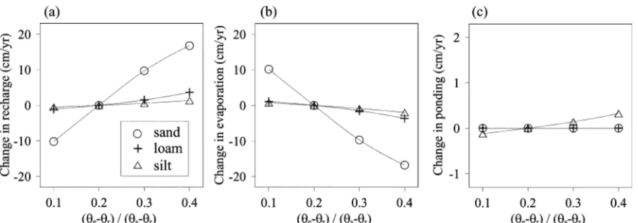
The threshold water content of maximum evaporation (θe) and the evaporation depth (ze) are considered for the sensi- tivity analysis. Each parameter is systematically changed within the plausible range while the other model parameters are fixed as given in Table 1, and its effects on the simula- tion results are examined. The parameter λ determining the weighting function of Eq. (17) is not considered in the sen- sitivity analysis, since the weighting function is confirmed to be insensitive to λ within several orders of magnitude.
Figure 13 shows the effect of varying the threshold water content (θe), which is represented as the equivalent effective saturation, on annual recharge, evaporation, and ponding averaged over the simulation period. Higher values of θe
implicitly indicate the tendency of soils yielding lower evap- Fig. 11. Effect of the water table depth on annual recharge and evaporation in relation to annual precipitation: (a) H=1 m and (b) H = 10 m.
Fig. 12. Simulated results for two-lay- ered model: (a) upper sand and lower silt layer and (b) upper silt and lower sand layer.