† Department of Civil Engineering, Kumoh National Institute of Technology (Corresponding Author : [email protected])
Delineation of Groundwater and Estimation of Seepage Velocity Using High-Resolution Distributed Fiber-Optic Sensor
Ki-Tae Chang†・ Quy-Ngoc Pham1)
Received: March 27th, 2015; Revised: April 20th, 2015; Accepted: May 15th, 2015
ABSTRACT : This study extends the Distributed Temperature Sensing (DTS) application to delineate the saturated zones in shallow sediment and evaluate the groundwater flow in both downward and upward directions. Dry, partially and fully saturated zones and water level in the subsurface can be recognized from this study. High resolution seepage velocity in vertical direction was estimated from the temperature data in the fully saturated zone. By a single profile, water level can be detected and seepage velocity in saturated zone can be estimated. Furthermore, thermal gradient analysis serves as a new technique to verify unsaturated and saturated zones in the subsurface. The vertical seepage velocity distribution in the recognized saturated zone is then analyzed with improvement of Bredehoeft and Papaopulos’ model. This new approach provides promising potential in real-time monitoring of groundwater movement.
Keywords : DTS, Seepage flow, Temperature profile, Monitoring, Groundwater Journal of the Korean Geo-Environmental Society
16(6): 39~43. (June, 2015) http://www.kges.or.kr
ISSN 1598-0820 DOI http://dx.doi.org/10.14481/jkges.2015.16.6.39
1. Introduction
Temperature profile has recently been proven as a useful tracer tool for appraising the groundwater movement in the subsurface. Many successful applications of heat tracer have been reported to identify surface water infiltration, interaction between surface water and groundwater, and flow patterns in the steam-bed aquifer sediments (Constantz, 1998; 2008;
Anderson, 2005; Hatch et al., 2006; Keery et al., 2007;
Schmidt et al., 2007; Vogt et al., 2010). Heat tracing involves analyzing temperature time series or profiles from temperature probes installed in the subsurface.
The temperature within sediment can be measured at discrete points by using conventional thermistors or by profiling the water column inside standpipe piezometers or existing casings.
With significant advances in temperature monitoring of distri- buted temperature sensors (TDS), it provides high resolution and fast measurement of temperature. Distributed temperature measurements using optical fibers bring the promise of improved spatial coverage and enable monitoring with high accuracy of 0.01 to 0.1℃.
Groundwater flow is governed by simultaneously coupled heat transfer and fluid flow models. The fundamentals of
using heat as a groundwater tracer have been developed since 1960s (Suzuki, 1960; Stallman, 1963; 1965; Bredehoeft &
Papaopulos, 1965), but recent work has significantly expanded the application to a variety of hydrogeological settings. In the field of engineering geology, potential application of heat tracing may have not yet recognized. The purpose of this study is to extend the application to works of geotechnical engineering works like embankment dam and dike or shallow sediment.
An experiment was built up to simulate temperature profile in laboratory by a soil column with DTS measurement system.
The high resolution measured temperature data from DTS system along soil column was utilized to map temperature profile in two dimensions of depth and time. Addition to the temperature profile, thermal gradient analysis of temperature profile was also carried out. Dry, partially and fully saturated medium could be recognized from the study. High resolution seepage velocity in vertical direction was estimated from temperature data in the fully saturated medium. By a single temperature profile, water level could be detected and seepage velocity in saturated medium could be estimated. This is a potential application in monitoring and evaluation of groundwater movement in near surface sediments.
2. Solution of One-Dimensional Heat Transfer Equation
Stallman (1963) developed the convection-conduction equation in the form of general partially differential equation (PDE) for three-dimensional coupled heat transport and fluid flow through fully saturated porous medium as:
(1)
where
: Temperature at any point at the time ;
, : Specific heat capacity of fluid and fluid-solid medium, respectively;
, : Mass density of fluid and fluid-solid medium, respectively;
,,: Seepage velocity component in the , and
direction, respectively;
,, : Cartesian coordinate;
t : time; and
k : Thermal conductivity.
In the case of coupled heat and groundwater flow in one dimension, the convection-conduction equation (1) in the vertical direction is reduced to:
, (2)
Many works have been done with application to steam-bed aquifer systems to investigate the interaction between surface water and groundwater (Hatch et al., 2006; Keery et al., 2007; Schmidt et al., 2007; Vogt et al., 2010). While these works focused only on downward infiltration, Bredehoeft and Papaopulos’ model (Bredehoeft & Papaopulos, 1965) involved with both upward and downward flow in the vertical direction.
In dealing with the vertical steady groundwater movement of an aquifer system, Bredehoeft & Papaopulos (1965) proposed an analytical solution for one-dimensional model with boundary conditions as:
, (3)
where
, (4)
: Temperature at the depth Z=0;
: Temperature at the depth Z;
: Temperature at depth L;
: Vertical length of temperature profile; and
: Vertical seepage velocity.
The left hand side of equation (3) is calculated from measured temperature data profile while the right hand side is a function of depth ratio (Z/L) and values of . The vertical downward or upward flow depends on the dimensionless values of , negative or positive, respectively. The vertical seepage velocity will be determined from equation (4) once value of is known. In order to solve equation (3), Bredehoeft & Papaopulos (1965) investigated the function f(Z/L, ) on the right hand side by building a graph of depth ratio (Z/L) versus f(Z/L, ) with different values of . The left hand side was superimposed with the depth ratio at the same scale and the value of was determined manually by best curve matching.
In this study, we investigate in optimizing approach the nonlinear solution of function
using iterative numerical method that involves to plug in trial values with condition (4):
, (5)
The convergence of the function (5) allows to estimate the values of (Brent, 2002). Seepage velocity can be computed with estimated value of as equation:
(6)
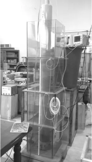
Fig. 1. Laboratory test configuration
Table 1. Physical properties of materials used in the test (Schön, 1998)
Materials Porosity Density Thermal conductivity
Specific heat capacity (-) (kg・m-3) (W・m-1・K-1) (J・kg-1・K-1)
Sand 0.3 2,650 2.4 733
Water 1,000 0.58 1,485
3. Thermal Gradient Analysis
The measured temperature distribution in spatial and temporal dimension can be described by a temperature profile map using a mesh grid system. Measured temperature data is assigned to the mesh grid system to develop high resolution temperature distribution map in depth and time series.
Temperature gradient map information including location, direction and magnitude can be derived from one grid. The arrow symbol points in the “downhill” direction and the length of the arrow depends on the magnitude, or steepness, of the slope. Direction of thermal gradient vector indicates the high temperature to the low temperature. Magnitude is indicated by arrow length. The steeper thermal gradient would have longer arrow. The location and direction of thermal gradient vector can be served as tracer of abnormal thermal variation. Magnitude and direction of thermal gradient vector may differentiate the heterogeneity of the medium.
4. Experimental Configuration
This test was carried out on the Joo-Mun-Jin standard sand with specification tabulated in Table 1. A one-dimensional sand column of 15 cm in diameter and 200 cm in length was used as a medium of transporting water flow coupled with heat transfer. The vertical fiber-optic sensor was located in the center of the sand column and consists of a 6-cm corrugated PVC tube wrapped by optical fiber. The optical fiber was protected against mechanical damage by covering it with an adhesive plastic film. The lower end of the sand column tube was closed with a plug and small holes in the plug allow water come in or out from bottom. The water fluctuation inside the sand column could be controlled by the water level in the water tank outside the sand column with assistance of a micro pump.
The optical fiber used for wrapping as communication cable has a multi-mode glass core, 0.05 mm thick, with a critical bending radius of 25 mm. The communication cable connects the fiber-optic vertical temperature sensor with the DTS control system. We used an OzOptics DTS system to measure the temperature along the fiber operating with 1 m sampling interval, 0.5 m spatial resolution and single-ended measurements averaged over 60 min.
5. Results and Discussion
Fig. 2 shows the temporal and spatial distribution of tem- perature along the sand column with temperature contour.
The measurement was performed continuously in 3 days.
Variation of temperature in the profile ranges from 11.70 to 13.60℃. The interface between sand and air, the water levels in the sand column and in the water tank were observed, as being indicated on the temperature profile.
Heat transfer in media with different thermal conductivity exhibits different behavior or tracer. In our test the heat
Fig. 2. High-resolution temperature distribution along the fiber-optic sensor profile in time and depth
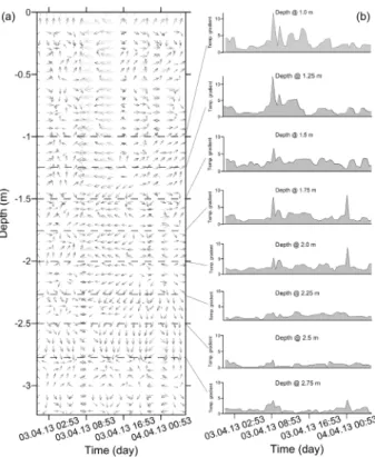
Fig. 3. Gradient thermal vector analysis: (a) Gradient vector distribution, (b) Thermal temperature magnitudes at different depth
transferred through different media of air, sand-air (dry sand), sand-water-air (partially saturated) and sand-water (fully saturated).
As shown in temperature profile of Fig. 2, the sand-air interface, water level in the sand column and water level outside in water tank can be recognized, in spite of some vagueness taken place. Water level in the tank went downward from -2.28 m to -2.38 m from surface with velocity of 11×10-5 cm/s, while water level in sand column appeared higher some 25 cm due to capillary action.
Addition to temperature distribution profile, thermal gradient analysis was also carried out. In the soil medium, the tem- perature transfer into void and matrix are different in magnitude and direction so that turbulences of thermal gradient vector.
The thermal gradient analysis of the temperature profile is presented in Fig. 3. The thermal gradient vector may be made field of the temperature profile is shown in Fig. 3(a), where vector’s magnitude and its color exhibits difference in temperature and vector’s direction indicates the temperature tendency. The direction, magnitude of thermal gradient vectors temporally demonstrates traces in term of thermal turbulence in the sand medium.
The thermal traces might, however, not reflect exactly the
texture of medium because of temperature changes in time but they contribute as an aid to interpret the soil medium.
The traces below the depth -2 m, especially around the depth -2.4 m can be account for the occurrence of partially saturated and fully saturated media. These traces also agree well with those appeared in temperature profile in Fig. 2.
The horizontal temperature gradient magnitude profiles at different depths are plotted in time series in Fig. 3(b). From the depth -1.75 m downward, temperature gradient magnitude is reduced compared to those above. This can be explained as the occurrence of higher moisture content from this depth downward. At the depth -2.25 m, the temperature gradient profile shows even smaller values.
In the fully saturated medium, the temperature turbulence and entropy become smaller so that a lower temperature gradient result in. In fully saturated medium, seepage flow simultaneously couples with heat transfer. The soil column from the depth of -2.5 m to -3.2 m is the target of seepage velocity estimation as illustrated in Fig. 2.
Fig. 4 shows contour of vertical seepage velocity distribution estimated automatically from Bredehoeft and Papaopulos’
model with numerical approach as equation 6. Positive values of seepage velocity exhibit downward flow corresponding to
Fig. 4. Contour of seepage velocity estimated from temperature profile [10-5 cm/s]
lowering down of water level in the water chamber at average velocity of 11×10-5 cm/s.
The values of seepage velocity range from of 5×10⁻⁵ to 20×10-5 cm/s. Some abnormal seepage velocity taken place might result from heterogeneity in the sediment or noisy temperature data produced from DTS system. Vogt et al.
(2010) reported that the DTS system may produce slightly noisy temperature data, especially in the first and last 15%
ends of the optical fiber.
6. Conclusions
Using distributed temperature sensing to quantify vertical flow seepage in steam-bed has successfully applied in previous works (Vogt et al., 2010; Gordon et al., 2012). The application limits to saturated medium as steam-bed sediment and a water infiltration in downward direction. In order to apply in near surface engineering works, this study extent the DTS application to delineate partially and saturated zones in shallow sediment and evaluate groundwater flow in both downward and upward directions. The vertical temperature measurement using optical fiber and DTS system provide high resolution temperature data for qualification of both unsaturated and saturated zones. Thermal gradient analysis serves as a new technique to differentiate unsaturated and saturated zones in the sediment. The vertical seepage velocity in the recognized saturated zone then analyzed with improve- ment of Bredehoeft and Papaopulos’ model. This new approach provides promising potential in real-time monitoring of groundwater movement.
Acknowledgement
This research was conducted during the sabbatical year supported by Kumoh National University of Technology.
References
1. Anderson, M. P. (2005), Heat as a ground water tracer, Ground water, Vol. 43, No. 6, pp. 951~968.
2. Bredehoeft, J. D. and Papaopulos, I. S. (1965), Rates of vertical groundwater movement estimated from the Earth’s thermal profile, Water Resources Research, Vol. 1, No. 2, pp. 325~328.
3. Brent, R. P. (2002), Algorithms for minimization without derivatives, 2nd ed., Mineola, New York: Dover Publ. Inc., pp.
206.
4. Constantz, J. (2008), Heat as a tracer to determine streambed water exchanges, Water Resources Research, Vol. 44, No. 4, pp. 243~257.
5. Constantz, J. (1998), Interaction between stream temperature, streamflow, and groundwater exchanges in alpine streams, Water Resources Research, Vol. 34, No. 7, pp. 1609~1615.
6. Gordon, R. P., Lautriz, L. K., Briggs, M. A. and McKenzie, J. M. (2012), Automated calculation of vertical pore-water flux from field temperature time series using the VFLUX method and computer program, Journal of Hydrology, Vol. 420, pp.
142~158.
7. Hatch, C. E., Fisher, A. T., Revenaugh, J. S., Constantz, J. and Ruehl, C. (2006), Quantifying surface water-groundwater interactions using time series analysis of streambed thermal records: Method development, Water Resources Research, Vol. 42, No. 10, pp.
1~14.
8. Keery, J., Binley, A., Crook, N. and Smith, J. W. N. (2007), Temporal and spatial variability of groundwater–surface water fluxes: Development and application of an analytical method using temperature time series, Journal of Hydrology, Vol. 336, No. 1, pp. 1~16.
9. Schmidt, C., Conant, B., Bayer-Raich, M. and Schirmer, M.
(2007), Evaluation and field-scale application of an analytical method to quantify groundwater discharge using mapped streambed temperatures, Journal of Hydrology, Vol. 347, pp. 292~307.
10. Schön, J. H. (1998), Physical properities of rocks - fundamentals and principles of petrophysics, 2nd ed., Pergamon, Oxford. pp.
583.
11. Stallman, R. W. (1963), Notes on the use of temperature data for computing ground-water velocity. In R. Bentall, ed. Methods of Collecting and Interpreting Ground-Water Data, Washington, DC: U.S. Geological Survey, pp. H36~H46.
12. Stallman, R. W. (1965), Steady one-dimensional fluid flow in a semi-infinite porous medium with sinusoidal surface temperature, Journal of Geophysical Research, Vol. 70, No. 12, pp. 2821~
2827.
13. Suzuki, S. (1960), Percolation measurements based on heat flow through soil with special reference to paddy fields, Journal of Geophysical Research, Vol. 65, No. 9, pp. 2883~2885.
14. Vogt, T., Schneider, P., Hahn-Woernle, L. and Cirpka, O. A.
(2010), Estimation of seepage rates in a losing stream by means of fiber-optic high-resolution vertical temperature profiling, Journal of Hydrology, Vol. 380, No. 1, pp. 154~164.
![Fig. 4. Contour of seepage velocity estimated from temperature profile [10 -5 cm/s]](https://thumb-ap.123doks.com/thumbv2/123dokinfo/5431007.429036/5.892.79.425.91.306/fig-contour-seepage-velocity-estimated-temperature-profile-cm.webp)