Comparison of Artificial Neural Network and Empirical Models to Determine Daily Reference Evapotranspiration

Comparison of Artificial Neural Network and Empirical Models to Determine Daily Reference Evapotranspiration

기준 일증발산량 산정을 위한 인공신경망 모델과 경험모델의 적용 및 비교

Yonghun Choi

⋅Minyoung Kim

⋅Susan O’Shaughnessy

⋅ Jonggil Jeon

⋅Youngjin Kim

⋅Weon Jung Song

최용훈⋅김민영⋅수잔 오샤네시⋅전종길⋅김영진⋅송원정

Abstract

The accurate estimation of reference crop evapotranspiration (ETo) is essential in irrigation water management to assess the time-dependent status of crop water use and irrigation scheduling. The importance of ETo has resulted in many direct and indirect methods to approximate its value and include pan evaporation, meteorological-based estimations, lysimetry, soil moisture depletion, and soil water balance equations. Artificial neural networks (ANNs) have been intensively implemented for process-based hydrologic modeling due to their superior performance using nonlinear modeling, pattern recognition, and classification. This study adapted two well-known ANN algorithms, Backpropagation neural network (BPNN) and Generalized regression neural network (GRNN), to evaluate their capability to accurately predict ETo using daily meteorological data. All data were obtained from two automated weather stations (Chupungryeong and Jangsu) located in the Yeongdong-gun (2002-2017) and Jangsu-gun (1988-2017), respectively.

Daily ETo was calculated using the Penman-Monteith equation as the benchmark method. These calculated values of ETo and corresponding meteorological data were separated into training, validation and test datasets. The performance of each ANN algorithm was evaluated against ETo

calculated from the benchmark method and multiple linear regression (MLR) model. The overall results showed that the BPNN algorithm performed best followed by the MLR and GRNN in a statistical sense and this could contribute to provide valuable information to farmers, water managers and policy makers for effective agricultural water governance.

Keywords: Reference evapotranspiration; penman-monteith equation; artificial neural networks (ANNs); backpropagation neural network (BPNN);

generalized-regression neural network (GRNN); multiple linear regression (MLR)

I. INTRODUCTION

Reference evapotranspiration (ET

) is one of the components

of the hydrologic cycle. Its precise estimation is critical to various agricultural and water management applications such as estimation of crop water requirements, irrigation scheduling, crop yield prediction, rainfall, runoff modeling, water resources planning and management, and water balance calculations (Allen et al., 1994; Kumar et al., 2002). Because of its significance, methods have been employed to measure ET

directly using lysimeters and pan evaporimeters, but they are time-consuming, require precise experimental setup and hours of maintenance to achieve reliable results (Igbadum et al., 2006). Micrometeorological methods using eddy covariance and scintillometry have also been employed to measure actual evapotranspiration, but they are expensive, complex and have limited applicability (Liu and Xu, 2017). Therefore, many studies have investigated indirect methods to estimate ET

and from these formulated equations using observed weather data as inputs. Examples of radiation-based methods include the Turc model, the Markkink, Jensen-Haise, Doorenbos and Pruitt, McGuinness and Bordne, Abtew, and Priestley-Taylor

a Post-doctoral researcher, Department of Agricultural Engineering, National Institute of Agricultural Sciences(NAS), Rural Development Administration(RDA)

b Agricultural Researcher, Department of Agricultural Engineering, National Institute of Agricultural Sciences(NAS), Rural Development Administration(RDA)

c Agricultural Engineer, Conservation and Production Research Laboratory, USDA Agricultural Research Service (USDA-ARS)

d Agricultural Researcher, Department of Agricultural Engineering, National Institute of Agricultural Sciences(NAS), Rural Development Administration(RDA)

e Agricultural Researcher, Department of Agricultural Engineering, National Institute of Agricultural Sciences(NAS), Rural Development Administration(RDA)

f Agricultural Researcher, Sangju Agricultural Technology Center

† Corresponding author

Tel.: +82-63-238-4156 Fax: +82-63-238-4145 E-mail: [email protected]

Received: July 17, 2018 Revised: September 27, 2018 Accepted: September 27, 2018

equations. Temperature-based methods include the Hargreaves, Thornthwaite, Romanenko, Hamon, Kharrufa, Linacre, and the Blaney-Criddle equations (Xu and Singh, 2000; Lang et al., 2017). Among the many numerical methods, the Penman-Monteith method (named here FAO56-PM) is the sole standard method recommended by the Food and Agricultural Organization (FAO) of the United Nations because it closely approximates ET

at the locations evaluated (Allen et al., 1994;

ASCE 2000).

The FAO56-PM equation accounts for aerodynamic as well as physiological parameters and requires large data input for estimating ET

, including geologic variables such as elevation and latitude, and meteorological variables such as minimum air temperature (T

), average air temperature (T

), maximum air temperature (T

), wind speed, relative humidity (RH) and sunshine hour. The high data demand of the FAO56-PM method provides for very accurate estimates but restricts its application in some data-lacking regions (Traore et al., 2008).

Over the past two decades, Artificial Neural Networks (ANNs) have been used extensively because of their ability to map input-output relationships without any understanding of physical processes and, therefore, can solve problems that are not amenable to conventional statistical or mathematical methods (Aytek et al., 2009). They are capable of learning and generalizing from examples to produce meaningful solutions to problems, even when input data contain errors or are incomplete. ANN

can also find adaptive solutions over time to compensate for changing circumstances, and process information rapidly (Jain et al., 2008; Rudd et al., 2014). Due to their capability of mapping non-linear relationships under any complex circumstance, ANNs have been widely used in diverse fields including hydrological modeling (Singh, 1988; Dawson and Wilby, 1998; Kim et al., 2008), streamflow prediction (Sahoo and Ray, 2006), suspended sediment modeling (Kişi, 2005), evapotranspiration modeling (Kumar et al., 2002), system dynamics (Azadeh et al., 2013), fault diagnosis and control (Koivo, 1994), pattern recognition (Basu et al., 2010), and financial forecasting (Kaastra and Boyd, 1996).

Despite many ANN applications, there are only a few studies that report on its use to predict ET

. Landeras et al. (2008) compared ANNs with ET

approximated by the FAO56-PM method for various locations in Spain. Seven ANNs with different input combinations were used and compared with ten empirical and semi-empirical ET

calculations. This study

showed that ANNs performed better than the locally calibrated ET

equations, so ANNs could be recommended in most situations if there is a deficiency in some of the meteorological sensors typically used in the FAO56-PM equation, such as solar radiation, vapor pressure, wind speed and relative humidity data (FAO, 1998). Antonopoulos et al. (2017) compared ET

estimations derived from ANNs and compared the values with the Priestly-Taylor, Makkink, and Hargreaves methods for one location in Greece. The data set of four variables, temperature, solar radiation, wind speed and relative humidity, was for a four-year period. They reported that the Priestley-Taylor and Makkink methods correlated well with the ANN model (correlation coefficients ranged from 0.955 to 0.986). However, the Hargreaves method over-estimated higher values of ET

. The RMSE from their investigations compared with the historical ET

calculations were rather larger and demonstrated that the model estimated ET

with the RMSE ranging from 0.574 to 1.33 mm/day. Importantly, Landeras et al. (2008) reports that the optimal ANN architecture varied by location.

According to the previous studies, the major problem when dealing with estimating evapotranspiration process is its complex and nonlinear dynamic, which means that it is favorable if there is sufficiently enough data available.

However, the situations are not always in that way. Therefore, this study was initiated to develop ANN model to accurately predict ET

and further utilize for irrigation scheduling even though there are limited and/or less available data. To cope with this, as the first step, this study assessed the performance of ANN using rich data accessible from automated weather stations operated by the Korea Meteorological Administration;

investigated the accuracy of ANN algorithms compared with the empirical model (Multiple Linear Regression); and determined the benefit or disadvantage of ANN models with two different computational algorithms in estimating ET

.

II. MATERIALS AND METHODS 1. Data collection and ET

calculation

Six daily meteorological data, average air temperature (T

,

°C), minimum and maximum air temperature (T

and T

,

°C), relative humidity (RH, %), wind speed (WS, m/s) and

sunshine hour (SH, hr), were obtained from the Chupungryeong

weather station, Yeongdong-gun, Gyeongbuk-province (Lat. 36

˚25’N, Long. 128˚09’E, 96.2 m above sea level) and the Jangsu weather station, Jangsu-gun, Jeonbuk-province (Lat. 35˚

39’N, Long. 127˚31’E, 406.5 m above sea level). The data from two weather stations covered 2002 to 2017 (15 years) and 1988 to 2017 (30 years), respectively.

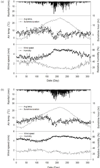
Figure 1 illustrates the distribution of multi-year mean data for T

, T

, T

, RH, WS, and SH. In Yeongdong, annual mean temperature, wind speed, relative humidity and sunshine hour were 12.7

C (-15.8∼ 37.2

C), 1.7 m/s (maximum of 7.2 m/s), 64.6% (17.5∼100%), and 6.0 hr (maximum of 13.6 hr), respectively. Annual mean temperature, wind speed, relative humidity and sunshine hour in Jangsu were 10.7

C (-25.8∼

34.7

C), 1.7 m/s (maximum of 7.6 m/s), 73.9% (30.4∼100%),

and 5.8 hr (maximum of 12.9 hr), respectively. The annual mean rainfall in Yeongdong and Jangsu were 1,151 mm and 1,457 mm, respectively, which were 200 mm and 100 mm less than the mean annual rainfall across the country.

In this study, ET

calculated with the FAO56-PM (equation 1) was used as the benchmark output value. The characteristics of a hypothetical reference crop (height = 0.12 m, surface resistance = 70 s/m, and albedo = 0.23) were adopted.

(1)

where, ET

is the daily reference crop evapotranspiration (mm/day), R

is the net radiation (MJ/m

⋅day), u

is the mean wind speed at 2 m above soil surface (m/s), T is the mean air temperature (°C), G is the soil heat flux density at the soil surface (MJ/m

⋅day), e

is the saturation vapor pressure (kPa), e

is the actual vapor pressure (kPa), Δ is the s lope of the saturation vapor pressure-temperature curve (kPa/°C), γ is the psychrometric constant (kPa/°C).

Sunshine hour, which is generally provided from two automated weather stations in the Korea Meteorological Administration, was converted to net solar radiation (SR) using the Angstrom-Prescott equation (2) (de Medeiros et al., 2017) in order to use the Penman-Monteith equation. The coefficients a (0.25) and b (0.5) for the Angstrom-Prescott equation, which are dependent on the physical characteristics of the atmospheric layer and influenced by local latitude, altitude and seasonal variability (e.g., rainfall, wind speed, relative humidity), were adopted (FAO, 1998)

(2)

where, H is daily global radiation on a horizontal surface (MJ/m

⋅day), H

is daily extraterrestrial radiation on a horizontal surface (MJ/m

⋅day), n is the daily number of hours of bright sunshine, and N is daily maximum number of hours of sunshine hour.

Reference crop evapotranspiration is the potential amount of water used by a crop, while actual evapotranspiration (ET

) of a well-watered crop is estimated by multiplying ET

by a crop coefficient (K

). Crop coefficients are crop and region specific.

Fig. 1 Multi-year daily climate characteristics of study area (a: Yeongdong, b: Jangsu)

They vary according to the growth stage of the crop and are determined under standard growing conditions, which is involve disease-free, well-fertilized and well-watered management (Allen et al., 1998). A detailed explanation of the theory of ET

is presented by Allen and FAO (1998).

In this study, daily values of T

, T

, T

, RH, WS and SR were used to compute ET

using the FAO56-PM equation which was coded into an Excel Spreadsheet. Daily results from the ANN and MLR models were compared against these approximated ET

values.

2. Multiple Linear Regression Analysis (MLR) Multiple linear regression techniques can be used to model evapotranspiration in terms of the local climatological parameters. The general purpose of the MLR model is to learn more about the relationship between several independent or predictor variables and a dependent or criterion variable. The general form of the regression equation is as follows (Kahane, 2008):

(3)

where, y: dependent variable, x

(i=1, 2, …, k): ith independent variables, b

: ith coefficient corresponding to x

, b

: intercept and k: number of observations.

In the multiple linear regression analysis, the values of ET

were used as the dependent variable and T

, T

, T

, RH, WS and SH were used as independent variables to derive the coefficients in the multiple linear regression model.

3. Artificial Neural Network Models:

Backpropagation neural network (BPNN) and Generalized regression neural network (GRNN) Artificial Neural Networks (ANNs) have universal approximation capabilities, which enable them to solve given differential equations possessing unsupervised error.

Backpropagation and Generalized Regression Neural Network models, two well-known feed-forward neural network techniques, were evaluated in this study.

The multilayer perceptron (MLP) is the most common, effective and successful neural network architecture which uses a supervised learning technique called Backpropagation (BP)

algorithm. Backpropagation neural network (BPNN) performs parallel training for improving the efficiency of MLP networks, derives the network error which is fed back into the network model and used to adjust the weights (Kecman, 2001; Mia et al., 2015). Adjustable weights are used to connect the nodes between adjacent layers and optimized by the training algorithm to obtain the desired results. Through that process, the error in prediction decreases with each iteration and succeeds when the neural network model reaches the specified level of accuracy, producing the desired outputs (Kim et al., 2008). A three-layer learning network used in this study consists of an input layer, one hidden layer and an output layer (Fig. 2).

To achieve the best performance model, the governing factors in BPNN, such as the number of hidden layers, the number of hidden processing elements (PEs), the transfer function (e.g., sigmoid, tan-sigmoid), learning algorithms (e.g., Delta, extended DBD), and learning parameters (e.g., learning rate, momentum factor, initial weights), were evaluated. Depending on the problem being solved, the success of training varies with selected factors. A trial-and-error procedure is normally preferred. Detailed information about each parameter (definition, function, range, etc.) is provided in Basheer and Hajmeer (2000) and Maier and Dandy (2000).

The generalized regression neural network (GRNN), is categorically a probabilistic neural network (PNN) model, which contains a neural network architecture that can solve any function approximation problem if sufficient data are made available. The main function of a GRNN is to estimate a linear or nonlinear regression surface on independent variables, i.e., the network computes the most probable value of an output y given only training x (Specht, 1991), where y is output and x is input.

Figure 2 is a schematic of the GRNN architecture with four

layers: an input layer, a hidden layer (pattern layer), a

summation layer, and an output layer which are connected in

sequence. In the pattern layer, each neuron presents a training

pattern and its output. In the summation layer there are two

different parts, a single division unit and a summation unit. This

layer performs a normalization of the output set along with the

output layer. In training the network, radial basis and linear

activation functions are used in hidden and output layers. Each

pattern layer unit is connected to the two neurons in the

summation layer, S and D. The S summation neuron computes

the sum of the weighted response of the pattern layer, while

the D summation neuron is used to calculate un-weighted outputs of pattern neurons. The output layer merely divides the output of each S-summation neuron by that of each D-summation neuron, yielding the predicted value y(x) to an unknown input vector x as ;

(4)

(5)

The distance, D

, between the training sample and the point of prediction, is used as a measure of how well each training sample can represent the position of the prediction, x. The smoothing factor  is a very important parameter of GRNN.

When a smoothing factor approaches 1, the network’s ability to generalize will be increased and the error of prediction degraded. In contrast, when a smoothing factor approaches 0, it degrades the network’s ability to generalize, or make predictions at all (Specht, 1991). Therefore, the optimum smoothing factor for the GRNN model should be determined empirically (Kim et al., 2011). More details on GRNN and its computational parameters are provided in Specht (1991).

4. Data processing and ANN computational procedures

In ANN computation, careful consideration should be given to choose suitable data that adequately represent the characteristics critical to the physical processes because networks trained with such data achieve higher generalization

capability. To accomplish this, the total of 5,830 and 10,944 data points for Yeongdong and Jangsu were divided into three subsets: a training set (62%), a validation set (8%) and a test set (30%).

Daily meteorological data, T

, T

, T

, RH, WS and SH, were selected as inputs and corresponding ET

values derived using the FAO56-PM method were used as output (desired) data. Because the input and output data consisted of different parameters with various physical meanings, units, and ranges, it was necessary to ensure that all variables receive equal attention during the training process. Therefore the data were normalized within the range from 0 to 1 using the following Min-Max normalization method:

(6)

where, Y

= the normalized dimensionless data of the specific input node; Y

= the measured/estimated data of the specific input node; Y

= the minimum data of the specific input node;

and Y

= the maximum data of the specific input node.

A PC-based neural network application software,

NeuralWorks Professional II/Plus (Neuralworks

, Pennsylvania,

USA) used in this study, allows the user to adjust key network

and training parameters in BPNN and GRNN. For example, the

number of hidden layers, Processing elements (PEs) in the

hidden layer, the momentum value, the learning rule (variation

of BP), the normalization technique, and the transfer function

in BPNN and the number of patterns, the reset factor, the radius

of influence, the sigma scale, and the sigma exponent in GRNN

can be adjusted. Modifications are performed to determine the best combination for solving the particular problem. Given the number of possible parameter combinations, the possibility of finding the correct combination of parameter settings, given a random starting point, is unlikely and is based primarily on chance (Kim et al., 2008).

Model convergence was based on the error function and exhibited any deviation between the predictions taken from corresponding target output values as the sum of the squares of the deviations. Training proceeded until the error was reduced to a desired minimum and the most commonly used stopping criterion our neural network training was the sum-of-squared-error (SSE), calculated for the training or test subsets as:

(7)

where, A

and T

are the actual and target solutions of the ith output node on the pth example, N is the number of training examples, and M is the number of output nodes (Basheer and Hajmeer, 2000).

5. Performance evaluation criteria

The performance of the BPNN, GRNN and MLR models were evaluated by comparing their predictive accuracies with the benchmark ET

values. The performance was characterized based on the following statistical criteria; R (correlation coefficient), R

(coefficient of determination), RMSE (root mean square error), E (Nash-Sutcliffe efficiency) and MAE (mean absolute error). The coefficient of determination (R

) and the residual mean square or root mean square error (RMSE) explain the proportion of variance and the residual variance between the ET

values estimated by FAO56-PM and ANN (MLR) models. Values of R

vary between 0 and 1, with higher values indicating less variance, and the values greater than 0.5 typically considered acceptable (Nash and Sutcliffe, 1970). The mean absolute error (MAE), as a measure of accuracy, takes the absolute value of the difference between ET

values. Model efficiency (E) is defined as one minus the sum of absolute squared differences between simulated and measured values, normalized by the variance of measured values during the period under investigation. The range of E lies between -∞ and

1.0 (perfect fit). An efficiency value between 0 and 1 is generally viewed as an acceptable level of performance (Nash and Sutcliffe, 1970). Efficiency lower than zero indicates that the mean value of the observed time series would be a better predictor than the model and denotes unacceptable performance (Moriasi, et al., 2007).

(8)

(9)

(10)

(11)

(12)

where, and represent the FAO56-PM estimate and its average for ith value; and represent the ANNs (MLR) computed value and its average for ith value; N represents the number of data considered.

III. RESULTS AND DISCUSSION 1. Reference evapotranspiration

In the present investigation, daily observation of T

, T

, T

, RH, WS and SR (derived from SH) were used to estimate ET

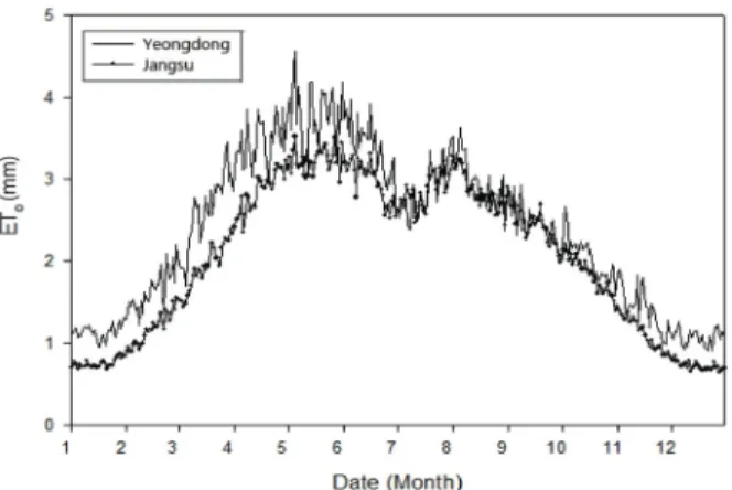
. The temporal trend of ET

showed that ET

in Yeongdong was approximately 1.3 times greater compared with ET

in Jangsu until July, and then after November. However, during August through October, ET

data were somewhat similar in both locations. An increase in rainfall and a decrease in SH resulted in a sudden drop in ET

during early July (Fig. 3).

The correlation between the six meteorological parameters used in this study with ET

are presented in Table 1. In Yeongdong, T

and T

had high correlations with ET

followed by SH, T

, RH and WS, but the correlation among

T

, T

and SH were not significantly different. Similarly, in Jangsu, T

and T

had high correlation with ET

. However, for the remaining parameters, the order of correlation (from highest to lowest) to ET

was T

, SH, RH and WS.

Table 1 indicated that RH consistently showed a negative correlation with ET

. On the contrary, T

, T

, T

, and SH had strong positive correlations with ET

. Analysis demonstrated that the impact of WS on the estimation of ET

was not significant in this study. However, Liu et al. (2014) showed that ET

decreases as WS decreases, and that sensitivities of ET

to WS is larger in humid regions than drier regions. In this study, although SH was significantly correlated with ET

, it was not the dominant parameter, especially in Jangsu, which is inconsistent with a study by Jun et al. (2012).

2. Development and comparison between ANNs and MLR models

The successful development of a BPNN model depends on several computational parameters, for example, multiple hidden layers, multiple neurons in a hidden layer, a momentum, a learning coefficient ratio, a learning rule and a transfer function.

Too few and too many neurons contribute to under-fitting and over-fitting problems, respectively. However, there is no

guiding rule to determine how many neurons in the hidden layer would work best upfront (Kecman, 2001). Therefore, the trial-and-error technique was applied by increasing the number of hidden layers and the number of neurons in the hidden layer until a small acceptable value of error and a high acceptable value of R

were achieved.

Our analyses with ET

revealed that the performance criteria for the best BPNN model for both locatoins had the architecture of 6-6-1, which had one input layer of 6 neurons, one hidden layer of 6 neurons and one output layer of 1 neuron. The momentum and learning coefficient ratios were initially set to 0.4 and 0.5, respectively. However, they were manipulated at 10 levels (increasing/decreasing by 0.1 from 0.0 to 1.0) in an effort to find the best configuration. The optimal momentum and learning coefficient rations were finally determined to be 0.1 and 0.7 for Yeongdong and 0.4 and 0.5 for Jangsu, respectively. In addition, this study adopted the Delta learning rule with the Tanh transfer function, which adjusts the weight of neurons by calculating the gradient of the loss function (i.e., gradient descent optimization algorithm).

The statistical analysis of data showed a close relationship between ET

calculated using the FAO56-PM equation and ET

simulated using the BPNN model; R

and E were 0.947 and 0.964, respectively, for Yeongdong and 0.962 and 0.962, respectively, for Jangsu, which indicated a high goodness-of-fit for both models for both locations. The RMSE and MAE were 0.057 and 0.010 (mm/day), respectively, for Yeongdong and 0.034 and 0.004 (mm/day), respectively, for Jangsu (Table 2).

The 1:1 graphical comparison between the estimated and simulated ET

shows a very high performance of the BPNN model (Fig. 4).

In comparison to BPNN, the GRNN architecture had a relatively simple and static structure, and there were no training parameters such as the optimum number of hidden layers or its neurons, momentum, learning rule and transfer (Ortiz-Rodríguez et al., 2013). The only significant parameter

Yeongdong and Jangsu

Region Tavg Tmin Tmax WS RH SH

ETo (Yeongdong) 0.62 0.51 0.68 0.07 -0.35 0.62

ETo (Jangsu) 0.75 0.65 0.79 0.09 -0.29 0.51

Note: Tavg= average air temperature, Tmin= minimum air temperature, Tmax= maximum air temperature, WS = wind speed, RH = relative humidity, SH = sunshine hour

Table 1 Correlation coefficient between meteorological data and ETo in the study regions

in GRNN was a s moothing factor (σ) which was considered to be the size of the neuron’s region and was empirically determined to be its optimum value. High smoothing factors increase the network’s ability to generalize and degrade the error of prediction while low smoothing factors degrade the network’s ability to generalize and make predictions at all (Kişi, 2005). In this study, a range of smoothing factors and method for selecting the smoothing factors were tested to determine the optimum smoothing factor which could be calculated as a sigma exponent divided by the number of input units (NeuralWare, 1993a).

Statistically, the GRNN models performed relatively well and the network structure which provided the best training and test results was selected based on the highest coefficient of correlation. The network structures of GRNN were with 5 inputs and 1 output for both regions, but different smoothing factors were empirically determined to be 0.07 for Jangsu and 0.12 for

Yeongdong. A change in the smoothing factor was evaluated based on R

values and the response of the GRNN model accuracy. An increase in the smoothing factor resulted in a parabolic curve, which indicated that as the smoothing factor increased, the R

value also increased. However, in practical terms, the GRNN model under-estimated ET

during the warm periods and over-estimated the values during the cold periods.

Figure 5 shows the performance of GRNN in Yeongdong and Jangsu during the test period. The R

and E values were 0.860 and 0.692, respectively, for Yeongdong and 0.917 and 0.676, respectively, for Jangsu. The RMSE and MAE values were 0.166 and 0.032 (mm/day), respectively, for Yeongdong and 0.100 and 0.016 (mm/day), respectively, for Jangsu (Table 2).

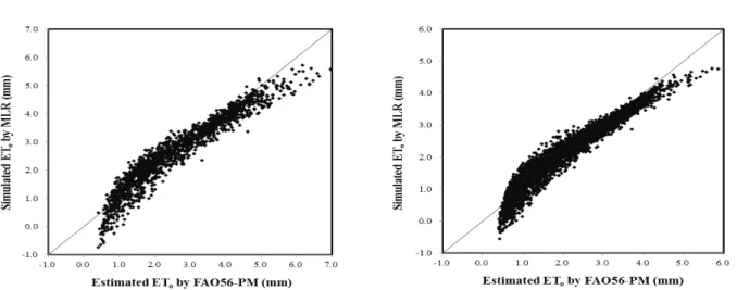
Figure 6 shows the performance of the MLR model in Yeongdong and Jangsu during the test period. This model performed better the GRNN models for the locations. The R

and E values were 0.900 and 0.897, respectively, for Yeongdong

Fig. 5 Scattering plot between FAO56-PM estimated and GRNN simulated results of daily ETo (Left: Yeongdong, Right: Jangsu)

and 0.897 and 0.883, respectively, for Jangsu. The RMSE and MAE were 0.096 and 0.018 (mm/day), respectively, for Yeongdong and 0.060 and 0.008 (mm/day), respectively, for Jangsu (Table 2). However, the MLR model generated negative values for the lowest values of ET

, which indicates that MLR is not an appropriate method to simulate ET

even though its correlation coefficients were higher. This result was consistent with the study by Doğan (2009) that found the same significant drawback of MLR models when used to estimate ET

.

IV. CONCLUSIONS

This study showed that six weather parameters, T

, T

, T

, WS, RH and SH, measured in Yeongdong and Jangsu were significantly correlated with ET

calculated for the areas using the FAO56-PM equation. All of these parameters were positively correlated with ET

with the exception of RH. It was also determined that WS in these regions was not significantly correlated with ET

. The present study also discussed the application and usefulness of the MLR and two different ANN modeling approaches in predicting ET

. The results from the

training and test datasets clearly demonstrated the ability of the BPNN model to predict daily values of ET

accurately using the climatic parameters, which were introduced as inputs to the chosen ANN models. Simulation results showed that the BPNN model outperformed the MLR and GRNN models.

The computational process to derive the optimal BPNN network models was somewhat complicated. Much time was spent determining the best values for several network parameters, such as the number of layers and neurons, choosing the type of activation functions and training algorithms, learning rates, and momentum values. The effective way of obtaining a good BPNN model was to use trial-and-error methods and thoroughly understand the theory of backpropagation.

Conversely, for the GRNN models, there was only one parameter, the smoothing factor, that was adjusted experimentally. However, the output estimates of the GRNN models during the warmest month, the time needed for additional irrigation, were low and would lead farmers to under-irrigate their crops. In the case of the MLR model, its negative estimates are a major drawback to estimating ET

accurately. This study also indicated that even though the BPNN

Region Model R R² RMSE E MAE

Yeongdong

BPNN 0.973 0.947 0.057 0.964 0.010

GRNN 0.928 0.860 0.166 0.692 0.032

MLR 0.949 0.900 0.096 0.897 0.018

Jangsu

BPNN 0.981 0.962 0.034 0.962 0.004

GRNN 0.958 0.918 0.100 0.676 0.016

MLR 0.947 0.897 0.059 0.883 0.008

Table 2 Statistical criteria for test data with ANN and MLR models

model required more time and effort to predict ET

compared with the GRNN and MLR models, it resulted in predicting the most accurate values of ET

. Although the predictions of the GRNN model were simpler and faster to obtain, they may not suit the needs of farmers or policy makers at critical crop growth stages and therefore, the modeler should take this into account before choosing the neural network algorithm to determine evapotranspiration.

Overall, the results were quite encouraging and suggested the usefulness of neural network-based modeling techniques for accurate prediction of ET

. As a beneficial attempt, the present study showed the possibility of estimating ET

with limited and/or lesser number of meteorological data as inputs, which is the limitation of the FAO56-PM equation, and could provide valuable information on irrigation scheduling in an easily accessible way. The forthcoming papers are underway and will be addressed these issues. Furthermore, accurate estimation of reference evapotranspiration using ANN modeling would contribute to establish in short- and long-term agricultural water resource plans against climate change.

ACKNOWLEDGEMENTS

This study was carried out with the support of the Research Program for Agricultural Science & Technology Development (Project No. PJ012686032018), National Institute of Agricultural Sciences (NAS), Rural Development Administration, Republic of Korea.

REFERENCES

1. Allen, R. G., M. Smith, A. Perrier, and L. S. Pereira, 1994.

An update for the definition of reference evapotranspiration.

ICID Bull 43(2): 1-92.

2. Allen, R. G., L. S. Pereira, D. Raes, and M. Smith, 1998.

Crop evapotranspiration - Guidelines for computing crop water requirements. FAO Irrigation and Drainage Paper, No 56 , FAO, Rome.

3. Allen, R. G. and Food and Agriculture Organization of the United Nations (FAO), 1998. Crop evapotranspiration:

guidelines for computing crop water requirements, 56-57, Food and Agricultural Organization of the United Nations, P. 300.

4. American Society of Civil Engineers (ASCE), 2000.

Standardization of Reference Evapotranspiration Task Committee, 2000.

5. Antonopoulos, V. Z. and A. V. Antonopoulos, 2017. Daily reference evapotranspiration estimates by artificial neural networks technique and empirical equations using limited input climate variables. Comp. Electron. Agric. 132: 86-96.

doi:10.1016/j.compag.2016.11.011

6. Aytek, A., A. Guven, M. I. Yuce, and H. Aksoy, 2009.

Reply to discussion of “an explicit neural network formulation for evapotranspiration”. Hydrological Sciences Journal 54(2): 389-393. doi:10.1623/hysj.54.2.389.

7. Azadeh, A., K. D. Shoushtari, M. Saberi, and E. Teimoury, 2013. An integrated artificial neural network and system dynamics approach in support of the viable system model to enhance industrial intelligence: the case of a large broiler industry. Systems Research and Behavior Science 31(2): 236-257. doi:10.1002/sres.2199.

8. Basheer I. A. and M. Hajmeer, 2000. Artificial neural networks: fundamentals, computing, design, and application.

J. Microbiol. Methods 43(1): 3-31.

9. Basu, J. K., D. Bhattacharyya, and T. H. Kim, 2010. Use of artificial neural network in pattern recognition.

International Journal of Software Engineering and its Applications 4(2): 23-43.

10. Dawson, C. W. and R. Wilby, 1998. An artificial neural network approach to rainfall-runoff modelling.

Hydrological Sciences Journal 43: 47-66. doi:10.1080/

02626669809492102

11. De Medeiros, F. J., C. M. e Silva, and B. G. Bezerra, 2017.

Calibration of Angstrom-Prescott equation to estimate daily solar radiation on Rio Grande do Norte State, Brazil.

Revista Brasileira de Meteorologia 32(3): 409-461.

12. Doğan, E., 2009. Reference evapotranspiration estimation using adaptive neuro-fuzzy inference systems. Irrigation And Drainage 58: 617-628. doi:10.1002/ird.445

13. Igbadum H. E, H. F. Mahoo, A. Tarimo, and B. A. Salim, 2006. Crop water productivity of an irrigated maize crop in Mkoji sub-catchment of Great Ruaha River Basin, Tanzania. Agricultural Water Management 85: 141-150.

doi:10.1016/j.agwat.2006.04.003

14. Food and Agriculture Organization of the United Nations

(FAO), 1998. Crop evapotranspiration: Guidelines for

computing crop water requirements. FAO irrigation and

drainage paper 56. Rome, Italy.

15. Kaastra, I. and M. Boyd, 1996. Designing a neural network for forecasting financial and economic time series.

Neurocomputing 10(3): 215-236.

16. Kahane, L. H., 2008. Regression Basics, 2

Ed. SAGE Publications Inc., Los Angeles, U.S.A.

17. Kecman, V., 2001. Learning and soft computing: Support vector machines, neural networks, and fuzzy logic model.

18. Kim, M., J. McGhee, S. Lee, and J. Thurston, 2011.

Comparative prediction schemes using conventional and advanced statistical analysis to predict microbial water quality in runoff form manured fields. Journal of Environmental Science and Health, Part A 46: 1392-1400.

19. Kim, M., C. Y. Choi, and C. P. Gerba, 2008. Source tracking of microbial intrusion in water system using artificial neural networks. Water Research 42(4-5): 1308-1314. doi:10.1016/

j.watres.2007.09.032

20. Kişi, O., 2005. Suspended sediment estimation using neuro-fuzzy and neural network approaches. Hydrological Sciences Journal 50(4): 683-696.

21. Koivo, H. N., 1994. Artificial neural networks in fault diagnosis and control. Control Engineering Practice 2(1):

89-101.

22. Kumar, M., N. S. Raghuwanshi, R. Singh, W. W. Wallender, and W. O. Pruitt, 2002. Estimating evapotranspiration using artificial neural network. Journal of Irrigation and Drainage Engineering ASCE 128(4): 224-233. doi:10.1061/

~ASCE!0733-9437~2002!128:4~224!

23. Jain, S. K., A. Sarkar, and V. Garg, 2008. Impact of declining trend of flow on Harike Wetland, India. Water Resources Management 22(4): 409-421.

24. Jun, W., X. Wang, M. Guo, and X. Xu, 2012, Impact of climate change on reference crop evapotranspiration in Chuxiong City, Yunnan Province. Procedia Earth and Planetary Science 5: 113-119.

25. Landeras, G., A. Ortiz-Barredo, and J. J. López, 2008.

Comparison of artificial neural network models and empirical and semi-empirical equations for daily reference evapotranspiration estimation in the Basque Country (Northern Spain). Agricultural Water Management 95(5):

553-565.

26. Lang, D., J. Zheng, J. Shi, F. Liao, X. Ma, W. Wang, X.

Chen, and M. Zhang, 2017. The comparative study of potential evapotranspiration estimation by eight methods with FAO Penman-Monteith method in Southwestern China. Water 9(734): 1-18.

27. Liu, S. and Z. Xu, 2017. Micrometeorological methods to determine evapotranspiration. Observation and Measurement 1-39.

28. Liu, X., X. J. Zhang, Q. Tang, and X. Z. Zhang, 2014.

Effects of surface wind speed decline on modeled hydrological conditions in China. Hydrology and Earth System Sciences 18(8): 2803-2813.

29. Maier, H. R. and G. C. Dandy, 2000. Neural networks for the prediction and forecasting of water resources variables:

a review of modeling issues and applications.

Environmental Modeling & Software 15: 101-124.

30. Mia, M. M. A., S. K. Biswas, M. C. Urmi, and A.

Siddique, 2015. An algorithm for training multilayer perceptron (MLP) for image reconstruction using neural network without overfitting. International Journal of Scientific & Technology Research 4(2): 271-275.

31. Moriasi, D. N., J. G. Arnold, M. W. Van Liew, R. L.

Bingner, and R. D. Harmel, 2007. Model evaluation guidelines for systematic quantification of accuracy in watershed simulations. Trans. ASABE 50: 885-900.

32. Nash, J. E. and J. V. Sutcliffe, 1970. River flow forecasting through conceptual models part I-A discussion of principles. Journal of Hydrology 10(3): 282-290.

33. NeuralWare, 1993. NeuralWorks Professional II/Plus:

Reference Guide, NeuralWare, Inc., Pittsburgh, PA, USA.

34. Ortiz-Rodríguez, J., M. Martinez-Blanco, J. Cervantes- Viramontes, and H. Vega-Carrillo, 2013. Robust design of artificial neural networks methodology in neutron spectrometry, In: K. Suzuki, ed. Artificial Neural Networks - Architectures and Applications, s.l.: InTech, pp. 83-111.

35. Rudd, K., G. Di Muro, and S. Ferrari, 2014. A constrained backpropagation approach for the adoptive solution of partial differential equations. IEEE Transactions on Neural Networks and Learning Systems 25(3): 571-584.

36. Sahoo, G. B. and C. Ray, 2006. Flow forecasting for a Hawaii stream using rating curves and neural networks.

Journal of Hydrology 317(1): 63-80.

37. Singh, V. P., 1988. Hydrology system rainfall-runoff modeling, vol. 1. Prentice Hall, Englewood Cliffs, New Jersey, USA.

38. Specht, D. F., 1991. A general regression neural network.

IEEE Transactions on Neural Networks 2(6): 568-576.

39. Traore, S., Y. M. Wang, and T. Kerh, 2008. Modeling

reference evapotranspiration by generalized regression

neural network in semiarid zone of Africa. WSEAS

Transactions on Information Science and Applications 5(6): 991-1000.

40. Xu, C. Y. and V. P. Singh, 2000. Evaluation and

generalization of radiation-based methods for calculating

evaporation. Hydrological Processes 14: 339-349.