AJCPP 2008 March 6-8, 2008, Gyeongju, Korea
Robust Fault Detection Based on Aero Engine LPV Model
Gou Linfeng1,Wang Xin2,ChenLiang3
(School of Power and Energy, Northwestern Polytechnical University, Xi’an Shannxi 710072, China)
Northwestern Polytechnical University, P.O.Box 188, Xi’an, 710072, China E-mail: [email protected]
Keywords: AJCPP, Propulsion, eigenstructure assignment, linear parameter varying model, fault detection filter Abstract
This paper develops an aero engine LPV mathematical model to exactly describe aero engine dynamic process characteristics, eliminate the effect of modeling error. Design FDF with eigenstructure assignment. The simulation results of turbofan engine control system sensor fault show that this method has good performance in focusing discrimination in fault signal with modeling eror, enhancing the robustness to unknown input, detecting accuracy is high and satisfiying real-time requirement.
1. Introduction
With the urgent demand for large thrust, long endurance and high reliability of modern aero power system. The foreign advanced aero engines all have state detection and fault diagnosis system, and takes on the trend of fire-flight-propulsion integration control. According to the special working conditions of the aero engine, the FADEC system must have rigorously considerable security and dependability, this demand sometimes seems to be more important than just improving control system performance. Once the control system runs error, it can be a disaster of the staff and financal resource.
In recent twenty years there has been growning research in fault diagnosis of the FADEC. For example, the ADIA of NASA Lewis research center[1]
etc. Many ways are analysis redundancy based on object steady linear model. But the aero engine is a typical non-linear system, its exterior and internal condition parameters quickly change in a large extent, the detection strategy lacking of robustness can't ensure engine’s best reliability. How to improve the robustness of fault detection has become research focus and a lot of research works have been done[2] [3] . Among the various approaches that have been proposed, the fault detection filter with eigenstructure assignment can improve the unsensitivity of parameter change and has received more and more attention[4].
The LPV(Linear Parameter Varying)object is an important type of time-varying system, its state equation is real-time measurable set and may be certain function of some time-varying parameters which can be predicted or be measured[5]. Because the dynamic character of aero engine is characterized by non-linear and time-varying, it can be expressed by LPV model which uses thermodynamics parameter or its variety rate, the LPV model can describe aero
engine’s dynamic process better. This paper uses Jacobian method to establish engine LPV model and make use of eigenstructure assignment to design the fault detection filter for detecting sensor fault and provides numberical examples.
2. The Establishment of Aero Engine’s LPV Model 2.1 Linear parameter varying system
The typical linear parameter varying system’s model can be described as follows:
⎩⎨
⎧
+
=
+
=
) ( )) ( ( ) ( )) ( ( ) (
) ( )) ( ( ) ( )) ( ( ) (
t u t D t x t C t y
t u t B t x t A t x
ρ ρ
ρ
& ρ (1)
Where
∑
∑
∑
∑
=
=
=
=
+
= +
=
+
= +
=
N k
k k N
k
k k
N k
k k N
k
k k
D t D
t D C t C
t C
B t B
t B A t A
t A
1 0 1
0
1 0 1
0
) ( ))
( ( , ) ( ))
( (
) ( ))
( ( , ) ( ))
( (
ρ ρ
ρ ρ
ρ ρ
ρ ρ
state vectorx(t)∈Rn, Output vectory(t)∈Rp, Input vector u(t)∈Rm , Ak,Bk,Ck,Dk
(k =0,1,LN ) are the N+1 partial models. ρ(t)is system parameter or exterior input(such as height, mach number etc) , and is boundary closed set.
Ifρ(t) is constant, the system is LTI and ρ(t) can be replaced by ρ.
2.2 The aero engine’s LPV model
The X turbofan engine is twin-duct, high thrust- weight ratio, birotary and afterburning. The engine’s non-linear model as follows:
⎩⎨
⎧
=
=
) , , (
) , , (
ρ ρ u x g y
u x
x& f (2)
If f(⋅) and g(⋅) are differentiable in flight envelope, we can use different methods to establish the partial linear model. If we have already known the state parameter, the LVP model can be constituted through little variation of state parameter and input parameter, or through a set of input-output data identification to get a set of linear model:
⎩⎨
⎧
− +
− +
−
=
−
− +
− +
−
=
) ( ) ( ) (
) ( ) ( ) (
0 0 0 0 0 0 0
0 0 0 0 0 0
ρ ρ ρ ρ
Q u u D x x C y y
P u u B x x
x& A (3)
Equation (3) expresses the feature of system (2) near the linear point, which usually is the steady balance points. This Paper uses the Jacobian method to develop model and its architecture presented in
35
AJCPP 2008 March 6-8, 2008, Gyeongju, Korea
Fig.1. To expase the non-linear model of aero engine at the point(x0,u0,ρ0)by Taylor series as follows:
u u x B x u x A u x f
u u u x x f x u x u f
x f x x x
Δ
⋅ +
Δ
⋅ +
∂ Δ +∂
∂ Δ +∂
= Δ +
=
) , , ( ) , , ( ) , , (
) , , ( ) , , ) ( , , (
0 0 0 0 0 0 0 0 0 0 0
0 0 0 0
0 0 0 0 0 0
ρ ρ
ρ
ρ ρ ρ
=
&
&
& (4)
Where Δx=x−x0 , Δu=u−u0 , subscript 0 represents an initial value.
Based on the partial model, use interior insert or fitting to get the coefficient matrix of Jacobian LVP model:
⎩⎨
⎧
Δ + Δ
= Δ
Δ + Δ
= Δ
u D x C y
u B x A x
) ( ) (
) ( ) (
ρ ρ
ρ
& ρ (5)
According to different ρto adjust different A, B, C, D.
(ρ) C )
(ρ A u
u0
Δu
y0y x0
x− x0
x && −
∫
(ρ) B
) (ρ D
- + +
+
Fig.1 The Jacobian LPV model principle diagram To solve Jacobian LPV model, the initial value
x0,y0andu0must be given.x&0can be non-zero value.
A problem demands attention. If using the interpolation of subsection constant function at the balanced points, it is essential to use variable transform to eliminate algebra rings for output y switch among the balanced points.
Computing the coefficient matrix by subsection linear interpolation through LPV model’s input and output relation will be better.
In state equation, the elements may make a great difference and become ill-conditioned matrix. To avoid greater calculation error, particularly in solving inverse matrix, matrix normalization must be done.
⎩⎨
⎧
+
=
+
=
n n n n n
n n n n n
U D X C Y
U B X A
X& (6)
where
x x
n N AN
A = −1 , Bn = Nx−1BN u ,Cn = Ny−1CN x ,
u y
n N DN
D = −1 .
Normalization matrix as follows:
⎥⎦
⎢ ⎤
⎣
=⎡
20 10
0 0 x
Nx x , ⎥
⎦
⎢ ⎤
⎣
=⎡
20 10
0 0 u
Nu u , ⎥
⎦
⎢ ⎤
⎣
=⎡
20 10
0 0 y Ny y
3. Design of Fault Detection Filter 3.1 Design principle
Consider the given system formulated explicitly in equation (7) below:
[ ]
⎭⎬
⎫ +
=
+ Δ
+
=
) ( ) ( ) (
) ( ) ( )
(
t Du t Cx t y
t Bu t x A A
x& t (7)
where the ΔA represents state matrix parameter perturbation. In order to improve the detection
robustness of uncertain input, the residual output unit add a weighting matrix.
Fig.2 The fault detection filter’s scheme with residual weighting matrix
Aim at the system (7), design a dynamic observer as follows:
[ ]
⎭⎬
⎫ +
=
− +
+
=
) ( ) ( ˆ ) ( ˆ
) ˆ( ) ( ) ( ) ˆ( ) ˆ(
t Du t x C t y
t y t y K t Bu t x A t
x& (8)
where K is the n × m dimensions gain matrix of the observer, xˆ(t)∈Rn is state estimation vector.
Rm
t
yˆ( )∈ is output estimation vector.
The state estimation error e(t) and weight output residual r(t) are
⎭⎬
⎫
−
=
−
=
)]
ˆ( ) ( [ ) (
) ( ˆ ) ( ) (
t y t y W t r
t x t x t
e (9)
where W ∈ Rp×mis a constant weighting matrix.
Residual output equation is
[ ]
[ ] ⎪⎭
⎪⎬
⎫
=
−
=
Δ +
−
=
−
−
− Δ +
=
−
=
) ( ) ( ˆ ) ( ) (
) ( ) ( ) (
) ˆ( ) ( ) ˆ( ) ( ) ( ) ˆ( ) ( ) (
t WCe t y t y W t r
t Ax t e KC A
t y t y K t x A t x A A t x t x t
e& & &
(10)
Defining Ac=A―KC, the Laplace transform of shift of output residual r(t) is
) ( )
( )
(s WC sI A 1 Ax s
r = − c − Δ (11)
Note from Eq.(10) that the effects of parameter variation can be decupled from the residual if correctly using eigenstructure assignment by weighting matrix W and K to make Eq.(11) as output-zeroing. Designing method is summaried as follows:
(1) Calcuate residual weighting matrix W to make WCΔA=0 .
(2) Determine the eigenstructure of the observer: the rows of H=WC should to be the p left
eigenvectors of the observer, the(n-p)left eigenvectors should to assure the rationality of model mtarix.
(3) Calculate the filter gain matrix K, satisfying the eigenstructure needs.
3.2 Fault detection
According to FDF’s output error residual vector has fix-directional characteristics, the fault event vector can be detected by comparing the direction of nomal vector and fault residual vector.
Defining minimal projection length of sensor fault vector:
System Sensor
Observer
W fault
residual r (t) y(t)
+
— u(t)
disturbance
36
AJCPP 2008 March 6-8, 2008, Gyeongju, Korea
2 2
*
) (
) ( ) (
k r
k r k
MLF j r − j
= (12) IfMLFj(j=1,2,..,m)is least, the No.j sensor is failure.
4. Numberical Example 4.1 The LPV model verification
Establish X turbofan engine LPV model with the high-compress speed Nch as adjusting variable, simulation can verify model’s dynamic tracking characteristic for low-compressor speed Ncl. Referenced model is the engine non-linear dynamic model, input variable is the fuel of main combustion chamber, sample cycle is 10ms.
From engine non-linear model, compute matrix A and B by subsection linear interpolation and three-order polynomial fitting at different speed. Fig.
3 and Fig.4 show the contrast.
0.80 0.82 0.84 0.86 0.88 0.90 0.92 0.94 0.96 0.98 1.00 -3.5
-3.0 -2.5 -2.0 -1.5 -1.0 -0.5 0.0 0.5
A22 A21 A12
A11
subsection linear interpolation three-order polynomial fitting
Matrix A elements
Nch
Fig.3 Matrix A elements interpolation and fitting
0.80 0.82 0.84 0.86 0.88 0.90 0.92 0.94 0.96 0.98 1.00 1000
1200 1400 1600 1800 2000 2200 2400
subsection linear interpolation three-order polynomial fitting B11
B21
Matrix B elements
Nch
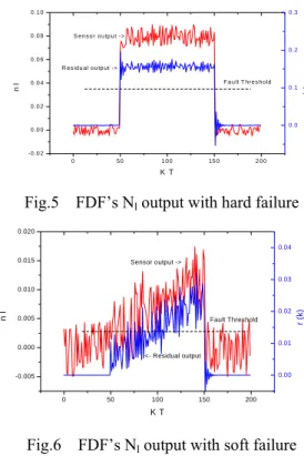
Fig.4 Matrix B elements interpolation and fitting 4.2 Sensor fault detection
Low-compressor speed sensor has occurred hard failure and soft failure, the FDF output and MLF value are shown as Fig.5 and Fig.6(State Point: H=8.0KM Ma=0.8). n ,l n ,h p ,*2 T4* sensor’s MLF constrast is shown as Table1.
0 5 0 1 0 0 1 5 0 2 0 0
-0 .0 2 0 .0 0 0 .0 2 0 .0 4 0 .0 6 0 .0 8 0 .1 0
K T
n l
0 .0 0 .1 0 .2 0 .3
F a u lt T h re s h o ld R e s id u a l o u tp u t ->
S e n s o r o u tp u t ->
r (k)
Fig.5 FDF’s Nl output with hard failure
0 50 100 150 200
-0.005 0.000 0.005 0.010 0.015 0.020
K T
n l
0.00 0.01 0.02 0.03 0.04
Fault Threshold
<- Residual output Sensor output ->
r (k)
Fig.6 FDF’s Nl output with soft failure
Sensor nlfault nhfault p*2fault T4*fault
MLF1 0.0516 0.2853 0.9901 0.9991 MLF2 0.1884 0.0733 0.9927 0.9927 MLF3 0.4639 0.3471 0.0149 0.9993 MLF4 0.9800 0.7181 0.9995 0.0297
Table 1 Four sensors MLF value contrast. If the sensor’s MLF is least, it’s in failure.
5. Conclusion
This paper provides an algorithm that designs FDF based on aero engine LPV model. From numberical simulation in the flight envelope, we can draw the following conclusions:
(1) LPV model that comparing with ordinary non-linear model can simlplify computational complexity, especailly in dynamic process, meanwhile accuracy is better.
(2) FDF based on LPV model can improve robustness in detection to unknown input and system parameters perturbation. Online fault detection time is not exceed four smpling periods.
References
1) John C DeLaat, Walter C Merrill.: Advanced Detection Isolation, and Accommodation of Sensor Failures in Turbofan Engine, Realtime Microcomputer Implementation, NASA 2925, 1990.
2) Ding S X, Jeinsch T, Frank P M.: A Unified Approach to the Optimization of Fault Detection Systems, IntJ Adaptive Control Signal Processing, 2000, 14 (7)
3) Niemann H, SaberiA, Stoorvogel.: Almost and Delayed Fault Detection: An Observer-based
37
AJCPP 2008 March 6-8, 2008, Gyeongju, Korea
Approach,Robust and Nonlinear Control, 1999, 9 (4)
4) Dohyeon Kim, Ookpyo Chun and Youdan Kim.:
On the robust fault detection and control reconfiguration via multipurpose observer, AIAA, 1997, 3780, pp755-761
5) Bei Lu,Fen Wu,and Sung Wan Kim.:
Switching LPV Control of An F-16 Aircraft via Controller State Reset,IEEE transactions on control systems technology,VOL.14,NO.2,
MARCH 2006
6) J. Park and G. Rizzoni.: An eigenstructure assignment algorithm for the Design of Fault Detection filters, IEEE Trans. Automat. Contr., vol 39, no. 7, pp 1521-1524, July 1994.
7) ZHONG Mai-ying, ZHANG Cheng-hui, DING S X.: Design of robust fault detection filterfor uncertain linear systems with modelling errors, Control Theory & Applications, 2003.5
8) YUAN Chun-fei, SUN Jian-guo, XIONG Zhi.: A Study of Propulsion Optimization Control Modes, Journal of Aerospace Power, 2004.1
38