Tsunami-induced Change Detection Using SAR Intensity and Texture Information Based on the Generalized Gaussian Mixture Model

(1)

Journal of the Korean Society of Surveying, Geodesy, Photogrammetry and Cartography Vol. 34, No. 2, 195-206, 2016

http://dx.doi.org/10.7848/ksgpc.2016.34.2.195

Tsunami-induced Change Detection Using SAR Intensity and Texture Information Based on the Generalized Gaussian Mixture Model

Jung, Min-young

¹⁾

ㆍKim, Yong-il

²⁾

Abstract

The remote sensing technique using SAR data have many advantages when applied to the disaster site due to its wide coverage and all-weather acquisition availability. Although a single-pol (polarimetric) SAR image cannot represent the land surface better than a quad-pol SAR image can, single-pol SAR data are worth using for disaster-induced change detection. In this paper, an automatic change detection method based on a mixture of GGDs (generalized Gaussian distribution) is proposed, and usability of the textural features and intensity is evaluated by using the proposed method. Three ALOS/PALSAR images were used in the experiments, and the study site was Norita City, which was affected by the 2011 Tohoku earthquake. The experiment results showed that the proposed automatic change detection method is practical for disaster sites where the large areas change.

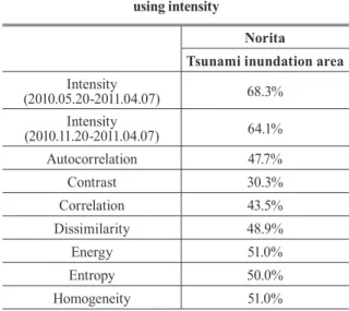
The intensity information is useful for detecting disaster-induced changes with a 68.3% g-mean, but the texture information is not. The autocorrelation and correlation show the interesting implication that they tend not to extract agricultural areas in the change detection map. Therefore, the final tsunami-induced change map is produced by the combination of three maps: one is derived from the intensity information and used as an initial map, and the others are derived from the textural information and used as auxiliary data.

Keywords : Synthetic Aperture Radar, Texture, Generalized Gaussian Mixture Model Expectation, Maximization, Tsunami-induced Change Detection

195 ISSN 1598-4850(Print) ISSN 2288-260X(Online) Original article

Received 2016. 04. 07, Revised 2016. 04. 17, Accepted 2016. 04. 27

1) Member, Dept. of Civil and Environmental Engineering, Seoul National University (E-mail: [email protected])

2) Corresponding Author, Member, Dept. of Civil and Environmental Engineering, Seoul National University (E-mail: [email protected])

This is an Open Access article distributed under the terms of the Creative Commons Attribution Non-Commercial License (http://

creativecommons.org/licenses/by-nc/3.0) which permits unrestricted non-commercial use, distribution, and reproduction in any medium, provided the original work is properly cited.

1. Introduction

After the occurrence of a severe disaster, rapid relief activities are extremely important for reducing the casualties.

For the urgent relief activities, analysis of the disaster site is needed, but it is usually very difﬁcult to immediately obtain information regarding the site through a ﬁeld survey.

Therefore, remote sensing data play an important role in the event of a disaster because remote sensors can observe the disaster site widely and rapidly. Among the various types of remote sensing data, SAR (Synthetic Aperture Radar) data are very efﬁcient because of their all-time and all-weather acquisition ability. Because the SAR sensor is an active sensor, which means that it generate its own signal unlike optic sensor, it can observe the surface during day or night.

In addition, as the signal of SAR sensor can penetrate clouds, SAR images can be acquired under all weather conditions (Zyl and Kim, 2011).

The previous research on detecting disaster-induced damage used the change detection method (Matsuoka and Yamazaki, 2004; Bovolo and Bruzzone, 2007; Gamba et al., 2007; Park et al., 2013). It compared the pre- and post-event images and extracted the changed areas as the damage areas. Matsuoka and Yamazaki (2004) calculated the backscattering coefﬁcient and the intensity correlation between two ERS (European Remote Sensing) satellite images and extracted areas with lower values as the damage areas. Gamba et al. (2007) detected them using the intensity and phase information of multitemporal ASAR (Advanced SAR) images with GIS data. Park et al. (2013) extracted

(2)

Journal of the Korean Society of Surveying, Geodesy, Photogrammetry and Cartography, Vol. 34, No. 2, 195-206, 2016

196

tsunami damage areas with the various polarimetric parameters of ALOS (Advanced Land Observation Satellite)/

PALSAR (Phased Array type L-band SAR) images, and revealed that quad-pol (polarimetric) SAR data can detect damage areas more accurately than single-pol SAR data can. The four types of scattering information (HH, HV, VH, and VV) in quad-pol SAR data are decomposed into various polarimetric parameters, and such parameters reﬂect the various characteristics of the land surface. Therefore, quad- pol data can well describe the features of the land surface.

The single-pol imaging mode, however, covers a greater area because of its wider swath width compared to the quad- pol mode (Ainsworth et al., 2009). Furthermore, much more pre-event images are available for comparison with the post- event images than quad-pol SAR data when a disaster occurs because a good number of single-pol SAR images have been obtained over the past decades. From this point of view, the change detection method using single-pol data is appropriate for disaster-induced change detection. Many disaster- induced damage detection cases using single-pol SAR data compared simple factors such as intensity or correlation between pre- and post-event images. To compensate for the insufﬁcient information on such factors, texture information can be applied. Texture information has been used in many previous studies for classiﬁcation, feature extraction, and change detection (Soh and Tsatsoulis, 1999; Zhu et al., 2012;

Kang et al., 2015). In particular, Kang et al. (2015) showed the potential use of texture information for urban change detection from VHR (very high resolution) SAR imagery.

Change detection for disaster-caused damage detection from SAR data should be automatic and unsupervised because prior knowledge such as ground truth information hardly exists in the disaster site. Unlike the use of optical data, automatic change detection using SAR data has been less exploited due to the SAR data’s speckle noise and geometry distortions (Bolvoro et al., 2013). Furthermore, because the statistical distribution is affected by the sensor type, the land cover type, etc., SAR data do not always follow the Gaussian distribution, which is traditionally envisaged in automatic thresholding algorithms like the K&I (Kittler and Illingworth, 1986) and Otsu (Otsu, 1975) methods. SAR intensity images generally follow various

gamma distributions such as Rayleigh, Nakagami, Weibull, etc. (Li et al., 2007). The major impediment, however, to using a generalized gamma distribution is its complexity and difﬁculty in parameter estimation (Gomes et al., 2008).

Therefore, automatic change detection based on a GGD (Generalized Gaussian distribution) can be an alternative due to its high ﬂexibility. The change detection method based on the GGD showed the proper results when it applied to SAR images (Bazi et al., 2009).

In this paper, an automatic change detection method based on the GGD is suggested for detecting disaster-induced damage areas. By applying the proposed change detection to intensity and texture images, a change map is produced. The only two single-pol SAR images are needed in the proposed method as it is considered that various data such as DEM (Digital Elevation Model) and optic images are not always available after the disaster. Texture images are ﬁrst generated by GLCM (Gray Level Co-occurrence Matrix). Statistical analysis based on the GGD is performed to DI (Difference Image) of each factor (intensity and textural features) through the EM (Expectation Maximization) algorithm. The ﬁnal change detection maps are derived from the statistical analysis results. In the following section, the methods of generating texture information and of automatically detecting change based on the GGD through the EM algorithm are explained in detail. The experiment results are reported and compared with one another in section 3, using the ALOS/PALSAR data of the 2011 Tohoku earthquake. Finally, conclusions are drawn in section 4.

2. Methodology

The proposed method consists of three steps: preprocessing, extracting the textural features, and automatic change detection. The preprocessing step includes geocoding, co- registration, and reducing speckle noise, in that sequence.

A transformed slant-range image, which is the natural result of radar-range measurement systems like the SAR system, is geocoded to a ground-range image, which is projected to a speciﬁc coordinate system. Co-registration and speckle ﬁltering are also performed for better change detection performance. In this paper, geo-coding and co-registration

(3)

Tsunami-induced Change Detection Using SAR Intensity and Texture Information Based on the Generalized Gaussian Mixture Model

197 were performed by the SNAP (Sentinel Application

Platform) which was downloaded through STEP (Science Toolbox Exploitation Platform) of ESA (European Space Agency) (http://step.esa.int/main/download/). The SNAP is the common architecture for all Sentinel Toolboxes which are the processing tools to support the diverse data including Sentinel-1, ERS-1 &2, ALOS/PALSAR, etc. The enhanced Lee ﬁlter with a 5×5-sized window was used for reducing the speckle noise. The other steps are explained below.

2.1 Extracting the textural features

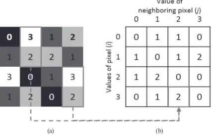
Texture information is about the spatial distribution of the pixel values in an image. GLCM is the most efficient method of representing the texture of an image (Lee et al., 2005). Three fundamental parameters must be defined when calculating the GLCM: the quantization levels, displacement (d), and orientation (α). GLCM is created by calculating the number of pixels with the gray value i, which are in the specific relationship to the pixels with the gray value j. The specific relationship is defined by distance (d) and orientation (α). Fig. 1 shows the creation of GLCM when the distance is set to 1 pixel and the orientation is set to 0°(vertical). The size of the resultant GLCM is affected by the size of the gray level of an image. In Fig. 1, the gray value varies from 0 to 3, and the size of the resultant GLCM is 4×4. If an image has n gray values from 0 to n-1, the size

of the resultant GLCM is n×n . Therefore, the size of the gray level must be quantized for efﬁcient calculation and for obtaining a desirable resultant texture information.

Haralick et al. (1973) suggested a set of 28 textural features using GLCM. In this paper, seven popular textural features were tested: autocorrelation, contrast, correlation, dissimilarity, energy (angular second moment), entropy, and homogeneity. The equations below deﬁne these features.

Autocorrelation =

Autocorrelation = ∑ ∑ 𝑖𝑖 𝑗𝑗 𝑝𝑝(𝑖𝑖, 𝑗𝑗)𝑖𝑖 𝑗𝑗 , (1)

where 𝑝𝑝(𝑖𝑖, 𝑗𝑗) is the value of the (𝑖𝑖, 𝑗𝑗)th cell in the normalized GLCM.

Contrast = ∑ ∑ (𝑖𝑖 − 𝑗𝑗)𝑖𝑖 𝑗𝑗 ² 𝑝𝑝(𝑖𝑖, 𝑗𝑗) (2)

Correlation =∑ ∑ 𝑖𝑖 𝑗𝑗 𝑝𝑝(𝑖𝑖,𝑗𝑗)−𝑖𝑖 𝑗𝑗 𝜇𝜇𝑖𝑖 𝜇𝜇𝑗𝑗 𝜎𝜎𝑖𝑖 𝜎𝜎𝑗𝑗 , (3)

where 𝜇𝜇𝑖𝑖, 𝜇𝜇𝑗𝑗, 𝜎𝜎𝑖𝑖, and 𝜎𝜎𝑗𝑗 are the means and standard deviations of row (i) and column (j).

Dissimilarity = ∑ ∑ |𝑖𝑖 − 𝑗𝑗| 𝑝𝑝(𝑖𝑖, 𝑗𝑗)_𝑖𝑖 _𝑗𝑗 (4)

Energy = ∑ ∑ 𝑝𝑝(𝑖𝑖, 𝑗𝑗)𝑖𝑖 𝑗𝑗 ²

(5)

Entropy = ∑ ∑ 𝑝𝑝(𝑖𝑖, 𝑗𝑗) log (𝑝𝑝(𝑖𝑖, 𝑗𝑗))_𝑖𝑖 _𝑗𝑗 (6)

If some relative frequencies 𝑝𝑝(𝑖𝑖, 𝑗𝑗) are zero, log (0) is not defined. Therefore, the set of (𝑖𝑖, 𝑗𝑗) where the value of 𝑝𝑝(𝑖𝑖, 𝑗𝑗) is 0 is excluded during the summation.

Homogeneity = ∑ ∑𝑖𝑖 𝑗𝑗_{1+(𝑖𝑖−𝑗𝑗)}^{𝑝𝑝(𝑖𝑖,𝑗𝑗)}2 (7)

𝑑𝑑 = log �^𝐼𝐼_𝐼𝐼^{𝑝𝑝𝑝𝑝𝑝𝑝𝑝𝑝}

𝑝𝑝𝑝𝑝𝑝𝑝�, (8)

where 𝐼𝐼𝑝𝑝𝑝𝑝𝑝𝑝, 𝐼𝐼𝑝𝑝𝑝𝑝𝑝𝑝𝑝𝑝 are the intensity values of the pre- and post-event images, respectively. The ratio method (𝑟𝑟 = 𝐼𝐼1/𝐼𝐼1) is desirable for SAR intensity images because unlike the difference method

(𝑑𝑑 = 𝐼𝐼1− 𝐼𝐼₀), it does p(𝑥𝑥|θ) =_{2𝛼𝛼Γ�}^𝛽𝛽1

𝛽𝛽�𝑒𝑒^−�^{|𝑥𝑥−𝜇𝜇|}^𝛼𝛼 ^�^𝛽𝛽,

, (1)

where p(i, j) is the value of the (i, j)th cell in the normalized GLCM.

Contrast =

Contrast = ∑ ∑ (𝑖𝑖 − 𝑗𝑗)_𝑖𝑖 _𝑗𝑗 ² 𝑝𝑝(𝑖𝑖, 𝑗𝑗) (2)

where 𝜇𝜇𝑖𝑖, 𝜇𝜇_𝑗𝑗, 𝜎𝜎_𝑖𝑖, and 𝜎𝜎_𝑗𝑗 are the means and standard deviations of row (i) and column (j).

Dissimilarity = ∑ ∑ |𝑖𝑖 − 𝑗𝑗| 𝑝𝑝(𝑖𝑖, 𝑗𝑗)𝑖𝑖 𝑗𝑗

(4)

(5)

Entropy = ∑ ∑ 𝑝𝑝(𝑖𝑖, 𝑗𝑗) log (𝑝𝑝(𝑖𝑖, 𝑗𝑗))𝑖𝑖 𝑗𝑗 (6)

(𝑑𝑑 = 𝐼𝐼1− 𝐼𝐼0), it does p(𝑥𝑥|θ) =_{2𝛼𝛼Γ�}^𝛽𝛽1

𝛽𝛽�𝑒𝑒^−�^{|𝑥𝑥−𝜇𝜇|}^𝛼𝛼 ^�

𝛽𝛽

,

(2)

Correlation =

(4)

(5)

(𝑑𝑑 = 𝐼𝐼1− 𝐼𝐼0), it does p(𝑥𝑥|θ) =_{2𝛼𝛼Γ�}^𝛽𝛽1 𝛽𝛽�𝑒𝑒^−�^{|𝑥𝑥−𝜇𝜇|}^𝛼𝛼 ^�

𝛽𝛽

,

, (3)

where μ_i, μ_j,σ_iand σ_j are the means and standard deviations of row (i) and column (j).

Dissimilarity =

(4)

(5)

where 𝐼𝐼𝑝𝑝𝑝𝑝𝑝𝑝, 𝐼𝐼_{𝑝𝑝𝑝𝑝𝑝𝑝𝑝𝑝} are the intensity values of the pre- and post-event images, respectively. The ratio method (𝑟𝑟 = 𝐼𝐼1/𝐼𝐼1) is desirable for SAR intensity images because unlike the difference method

𝛽𝛽

,

(4)

Energy =

Correlation =∑ ∑ 𝑖𝑖 𝑗𝑗 𝑝𝑝(𝑖𝑖,𝑗𝑗)−_𝑖𝑖 _𝑗𝑗 𝜇𝜇𝑖𝑖 𝜇𝜇𝑗𝑗 𝜎𝜎𝑖𝑖 𝜎𝜎𝑗𝑗 , (3)

Energy = ∑ ∑ 𝑝𝑝(𝑖𝑖, 𝑗𝑗)_𝑖𝑖 _𝑗𝑗 ² (5)

where 𝐼𝐼𝑝𝑝𝑝𝑝𝑝𝑝, 𝐼𝐼𝑝𝑝𝑝𝑝𝑝𝑝𝑝𝑝 are the intensity values of the pre- and post-event images, respectively. The ratio method (𝑟𝑟 = 𝐼𝐼1/𝐼𝐼₁) is desirable for SAR intensity images because unlike the difference method

𝛽𝛽

,

(5)

Entropy =

(5)

where 𝐼𝐼𝑝𝑝𝑝𝑝𝑝𝑝, 𝐼𝐼𝑝𝑝𝑝𝑝𝑝𝑝𝑝𝑝 are the intensity values of the pre- and post-event images, respectively. The ratio method (𝑟𝑟 = 𝐼𝐼1/𝐼𝐼₁) is desirable for SAR intensity images because unlike the difference method

𝛽𝛽

,

(6)

Fig. 1. Calculation of GLCM (distance=1; orientation=0°): (a) objective image; (b) GLCM

(a) (b)

(4)

Journal of the Korean Society of Surveying, Geodesy, Photogrammetry and Cartography, Vol. 34, No. 2, 195-206, 2016

198

If some relative frequencies p(i, j) are zero, log (0) is not deﬁned. Therefore, the set of (i, j) where the value of p(i, j) is 0 is excluded during the summation.

Homogeneity =

(5)

𝛽𝛽

,

(7)

2.2 Automatic change detection

A change detection method traditionally consists of two parts: DI generation and thresholding. As it was assumed, however, that the DI of SAR data follows the GGD, statistical modeling of the DI based on a mixture of GGDs using the EM algorithm was additionally performed before thresholding.

2.2.1 DI generation

The DI of intensity was directly calculated using the log- ratio method (Eq. (8)).

(4)

(5)

where 𝐼𝐼𝑝𝑝𝑝𝑝𝑝𝑝, 𝐼𝐼_{𝑝𝑝𝑝𝑝𝑝𝑝𝑝𝑝} are the intensity values of the pre- and post-event images, respectively. The ratio method (𝑟𝑟 = 𝐼𝐼1/𝐼𝐼1) is desirable for SAR intensity images because unlike the difference method

𝛽𝛽

, , (8)

where I_pre, I_postare the intensity values of the pre- and post-event images, respectively. The ratio method (r=I₁/ I₁) is desirable for SAR intensity images because unlike the difference method (d=I₁–I₀), it does not depend on the intensity level of the pixels and is very robust against calibration errors (Rignot et al., 1993). For the DI of textural images, log calculation was ﬁrst applied to the pre-processed images.

The textural features that were used in this paper were calculated by the GLCMs. The difference method is desirable for texture feature images.

2.2.2 Statistical modeling of DI (1) A mixture of GGDs

The Gaussian distribution, which is known as a normal distribution, is the most popular distribution in statistics (Nadarajah, 2005). When the Gaussian distribution is naturally generalized, it becomes a GGD. The pdf (probability density function) of GGD is given by (Elguebaly and Bouguila, 2011)

(4)

(5)

𝛽𝛽

,, (9)

where

(9)

where 𝑥𝑥 (𝑥𝑥 ∈ ℝ) is the random variable which is a gray value in this paper, and 𝜃𝜃 is the set of statistical parameters, including 𝜇𝜇, 𝛼𝛼, and 𝛽𝛽 which denote the mean, scale, and shape parameters, respectively. The Γ(∙) is the Gamma function. The shape parameter, 𝛽𝛽, determines the flatness of the p(𝑥𝑥) = ∑ P^𝑘𝑘𝑖𝑖=1 𝑖𝑖p(𝑥𝑥|𝜃𝜃𝑖𝑖),

(10)

where P𝑖𝑖 is the prior probabilities and 𝜃𝜃𝑖𝑖 is the set of statistical parameters associated with the ith L(𝑋𝑋|Θ) = ∏^𝑁𝑁𝑗𝑗=1𝑝𝑝(𝑥𝑥𝑗𝑗),

(11)

where 𝛩𝛩 refers to the entire set of parameters to be estimated. The EM algorithm considers the data incomplete and having a missing part. Therefore, each pixel, 𝑥𝑥𝑗𝑗, is associated with 𝑧𝑧𝑗𝑗 for applying the EM algorithm to the image, X, which means a hidden variable that indicates which distribution includes 𝑥𝑥𝑗𝑗. For example, if 𝑥𝑥𝑗𝑗 belongs to the ith distribution, 𝑧𝑧𝑗𝑗𝑖𝑖 is equal to 1. Otherwise, 𝑧𝑧𝑗𝑗𝑖𝑖 is equal to 0. The likelihood of a complete X is given by

L(X|Θ) = ∏𝑁𝑁 ∑^𝑘𝑘𝑖𝑖=1P𝑖𝑖p(𝑥𝑥𝑗𝑗|𝜃𝜃𝑖𝑖)^𝑧𝑧^{𝑗𝑗𝑗𝑗}

𝑗𝑗=1 .

(12)

The log-likelihood of Eq. (12) is expressed as

𝐿𝐿^∗(X, Z|Θ) = ∑𝑁𝑁 ∑^𝑘𝑘𝑖𝑖=1𝑧𝑧𝑖𝑖𝑗𝑗lnP𝑖𝑖p(𝑥𝑥𝑗𝑗|𝜃𝜃𝑖𝑖)

𝑗𝑗=1 ,

(13)

where Z is the set of 𝑧𝑧𝑗𝑗. Using Eq. (9), the log-likelihood of X is given by

𝐿𝐿^∗(X, Z|Θ) = ∑ ∑𝑁𝑁 𝑧𝑧𝑖𝑖𝑗𝑗lnP𝑖𝑖 𝑘𝑘 𝑗𝑗=1

𝑖𝑖=1 + ∑ ∑ 𝑧𝑧𝑖𝑖𝑗𝑗�ln𝛽𝛽𝑖𝑖− ln2 − ln𝛼𝛼𝑖𝑖− lnΓ �_𝛽𝛽¹

𝑗𝑗� − �^{|𝑥𝑥−𝜇𝜇|}_𝛼𝛼 �^𝛽𝛽�

𝑁𝑁𝑗𝑗=1

𝑘𝑘𝑖𝑖=1 .

(14)

Each 𝑧𝑧𝑖𝑖𝑗𝑗 can be replaced by its conditional expectation associated with 𝑥𝑥𝑗𝑗 and the parameters of is the random variable which is a gray

value in this paper, and θ is the set of statistical parameters, including μ, α and β which denote the mean, scale, and shape parameters, respectively. The

(9)

where 𝑥𝑥 (𝑥𝑥 ∈ ℝ) is the random variable which is a gray value in this paper, and 𝜃𝜃 is the set of statistical parameters, including 𝜇𝜇, 𝛼𝛼, and 𝛽𝛽 which denote the mean, scale, and shape parameters, respectively. The Γ(∙) is the Gamma function. The shape parameter, 𝛽𝛽, determines the flatness of the p(𝑥𝑥) = ∑ P^𝑘𝑘_𝑖𝑖=1 𝑖𝑖p(𝑥𝑥|𝜃𝜃𝑖𝑖),

(10)

where P𝑖𝑖 is the prior probabilities and 𝜃𝜃𝑖𝑖 is the set of statistical parameters associated with the ith L(𝑋𝑋|Θ) = ∏^𝑁𝑁_𝑗𝑗=1𝑝𝑝(𝑥𝑥𝑗𝑗),

(11)

L(X|Θ) = ∏^𝑁𝑁𝑗𝑗=1∑^𝑘𝑘_𝑖𝑖=1P𝑖𝑖p(𝑥𝑥𝑗𝑗|𝜃𝜃𝑖𝑖)^𝑧𝑧^{𝑗𝑗𝑗𝑗}. (12)

𝐿𝐿^∗(X, Z|Θ) = ∑^𝑁𝑁_𝑗𝑗=1∑^𝑘𝑘_𝑖𝑖=1𝑧𝑧𝑖𝑖𝑗𝑗lnP𝑖𝑖p(𝑥𝑥𝑗𝑗|𝜃𝜃𝑖𝑖), (13)

𝐿𝐿^∗(X, Z|Θ) = ∑^𝑘𝑘_𝑖𝑖=1∑^𝑁𝑁_𝑗𝑗=1𝑧𝑧_{𝑖𝑖𝑗𝑗}lnP_𝑖𝑖+ ∑ ∑ 𝑧𝑧_{𝑖𝑖𝑗𝑗}�ln𝛽𝛽𝑖𝑖− ln2 − ln𝛼𝛼_𝑖𝑖− lnΓ �_𝛽𝛽¹

𝑗𝑗� − �^{|𝑥𝑥−𝜇𝜇|}_𝛼𝛼 �^𝛽𝛽�

𝑁𝑁𝑗𝑗=1

(14)

Each 𝑧𝑧𝑖𝑖𝑗𝑗 can be replaced by its conditional expectation associated with 𝑥𝑥𝑗𝑗 and the parameters of is the Gamma function.

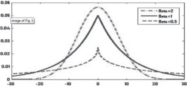
The shape parameter, β, determines the ﬂatness of the pdf (Fig.2). By changing the value of β, the GGD is made to include a variety of statistical distributions, such as the uniform, Gaussian, Laplacian, and impulsive distributions.

For example, when β = 2, the pdf is the Gaussian distribution, and when β = 1, the pdf is the Laplacian distribution. The ﬂexibility of the GGD is one of the reasons that many previous works adopted it.

It was assumed that the DI follows a mixture of two GGDs:

one for a class of changed pixels and the other for a class of unchanged pixels. If the random variable, x, follows a mixture of k GGDs, then pdf is represented as

(9)

where 𝑥𝑥 (𝑥𝑥 ∈ ℝ) is the random variable which is a gray value in this paper, and 𝜃𝜃 is the set of statistical parameters, including 𝜇𝜇, 𝛼𝛼, and 𝛽𝛽 which denote the mean, scale, and shape parameters, respectively. The Γ(∙) is the Gamma function. The shape parameter, 𝛽𝛽, determines the flatness of the p(𝑥𝑥) = ∑ P^𝑘𝑘_𝑖𝑖=1 𝑖𝑖p(𝑥𝑥|𝜃𝜃𝑖𝑖),

(10)

where P𝑖𝑖 is the prior probabilities and 𝜃𝜃𝑖𝑖 is the set of statistical parameters associated with the ith L(𝑋𝑋|Θ) = ∏^𝑁𝑁_𝑗𝑗=1𝑝𝑝(𝑥𝑥𝑗𝑗),

(11)

L(X|Θ) = ∏^𝑁𝑁_𝑗𝑗=1∑^𝑘𝑘_𝑖𝑖=1P𝑖𝑖p(𝑥𝑥𝑗𝑗|𝜃𝜃𝑖𝑖)^𝑧𝑧^{𝑗𝑗𝑗𝑗}. (12)

𝐿𝐿^∗(X, Z|Θ) = ∑^𝑁𝑁_𝑗𝑗=1∑^𝑘𝑘_𝑖𝑖=1𝑧𝑧𝑖𝑖𝑗𝑗lnP𝑖𝑖p(𝑥𝑥𝑗𝑗|𝜃𝜃𝑖𝑖), (13)

𝐿𝐿^∗(X, Z|Θ) = ∑ ∑𝑁𝑁 𝑧𝑧𝑖𝑖𝑗𝑗lnP𝑖𝑖 𝑘𝑘 𝑗𝑗=1

𝑖𝑖=1 + ∑ ∑ 𝑧𝑧𝑖𝑖𝑗𝑗�ln𝛽𝛽𝑖𝑖− ln2 − ln𝛼𝛼𝑖𝑖− lnΓ �_𝛽𝛽¹

𝑗𝑗� − �^{|𝑥𝑥−𝜇𝜇|}_𝛼𝛼 �^𝛽𝛽�

𝑁𝑁𝑗𝑗=1

(14)

Each 𝑧𝑧𝑖𝑖𝑗𝑗 can be replaced by its conditional expectation associated with 𝑥𝑥𝑗𝑗 and the parameters of , (10)

where P_i is the prior probabilities and θ_i is the set of statistical parameters associated with the ith distribution. It was noticed that an ith GGD has four unknown parameters:

P_i, μ_i,α_iand β_i. Therefore, modeling an image with a mixture of k GGDs means that 4k parameters should be estimated.

This problem can be solved by the maximizing the log- likelihood using the EM algorithm.

(2) EM algorithm

The EM algorithm (Dempster et al., 1977) is well known for the estimation of unknown parameters for a mixture

Fig. 2. GGDs with different shape parameter β (Elguebaly and Bouguila, 2011)