Investigation on the Applicability of Defocus Blur Variations to Depth Calculation Using Target Sheet Images Captured by a DSLR Camera
Seo, Suyoung
1)Abstract
Depth calculation of objects in a scene from images is one of the most studied processes in the fields of image processing, computer vision, and photogrammetry. Conventionally, depth is calculated using a pair of overlapped images captured at different view points. However, there have been studies to calculate depths from a single image. Theoretically, it is known to be possible to calculate depth using the diameter of CoC (Circle of Confusion) caused by defocus under the assumption of a thin lens model. Thus, this study aims to verify the validity of the thin lens model to calculate depth from edge blur amount which corresponds to the radius of CoC. For this study, a commercially available DSLR (Digital Single Lens Reflex) camera was used to capture a set of target sheets which had different edge contrasts. In order to find out the pattern of the variations of edge blur against varying combination of FD (Focusing Distance) and OD (Object Distance), the camera was set to varying FD and target sheet images were captured at varying OD under each FD. Then, the edge blur and edge displacement were estimated from edge slope profiles using a brute-force method. The experimental results show that the pattern of the variations of edge blur observed in the target images was apart from their corresponding theoretical amounts derived under the thin lens assumption but can still be utilized to calculate depth from a single image for the cases similar to the limited conditions experimented under which the tendency between FD and OD is manifest.
Keywords : Defocus, Blur, Target Sheet, Blur Variation, DSLR Camera, Depth Calculation
1. Introduction
Extraction of elevation or depth information of objects in a scene from images is one of the most fundamental processes in image processing, computer vision, and photogrammetry.
Typically, the extraction of those information is carried out using a pair of images which have overlapped regions only for which the 3-D information of objects can be extracted.
However, there have been attempts to extract depth information from a single image (Green et al., 2007; Zhou et al., 2009; Kim et al., 2012).
The types of blur observed in an image can be cartegorized into two types:
motion blur and defocus/out-of-focus blur. Firstly, motion blur is typically caused by movement of a camera or objects during camera exposure (Yuan et al., 2007;
Oliveira et al., 2014; Zhang and Hirakawa, 2015; Zhang and Hirakawa, 2016; Lu et al., 2016). The motion blur is typically estimated in the form of a blur kernel and the blur kernel is used in a deconvolution process for deblurring the images. Secondly, defocus blur is typically caused by the difference between FD (Focusing Distance) and OD (Object Distance). Many approaches have been proposed to identify the amount of defocus blur in images so that deblurring can be performed based on the blur amount (De et al., 2006; Cao et al., 2013; Hong et al., 2015; Chen and Shen, 2015; Zhang
Received 2020. 03. 18, Revised 2020. 04. 10, Accepted 2020. 04. 23
1) Member, Professor, Dept. of Civil Engineering, Kyungpook National University (E-mail: [email protected])
https://doi.org/10.7848/ksgpc.2020.38.2.109 Original article
This is an Open Access article distributed under the terms of the Creative Commons Attribution Non-Commercial License (http://
Journal of the Korean Society of Surveying, Geodesy, Photogrammetry and Cartography, Vol. 38, No. 2, 109-121, 2020
and Hirakawa, 2016). In addtion, the blur maps resulting from blur amount estimation were used for foreground/
background segmentation (Zhu et al., 2013). Furthermore, the approaches using a single image for depth information extraction are also typically based on the estimation of defocus blur (Green et al., 2007; Zhou et al., 2009; Kim et al., 2012).
In the estimation of defocus blur, it is needed to model the blur function. There have been two types of blur functions:
cylindrical function and Gaussian function. Cylindrical functions have been used to model the blur pattern caused by the camera aperture shape (Moghaddam, 2007; Wu and Lin, 2008; Sun et al., 2009; Oliveira et al., 2014; Gajjar and Zaveri, 2017). However, Gaussian functions appear to be more appropriate to model the blur because the blur shape observed in real images is more Gaussian-like than cylinder- like (Zhuo and Sim, 2011; Cao et al., 2013; Chen and Shen, 2015; Tang et al., 2013; Hong et al., 2015; Zhang and Hirakawa, 2016; Seo, 2017a; Seo, 2017b; Seo, 2018a; Seo, 2018b; Karaali and Jung, 2018).
After a blur function is modeled, its blur parameters are estimated in the subsequent process. The estimation of blur parameters was performed based on image reblurring and calculation of the ratio of gradients derived from different magnitudes of reblurring (Zhuo and Sim, 2011; Karaali and Jung, 2018). In addition, an estimation method was proposed based on fitting the logarithmic values of gradients to a quadratic polynomial (Hong et al., 2015). One of the problems of the Hong et al.‘s method is that the method cannot estimate the blur function with the full width of a gradient profile because it is impossible to calculate the logarithmic value of gradients when gradient values are less than or equal to 0. To resolve this problem, a brute-force estimation method was proposed in Seo (2018a).
In order to extract depth information from a single image, methods to modify camera systems were proposed (Green et al., 2007; Zhou et al., 2009; Kim et al., 2012). Although, the approaches showed a certain level of accuracy for depth estimation, one of the demerits of the approaches is the requirement of manipulation of the camera systems. A method to use images of a checkerboard with dots (Reuter et al., 2012) was proposed to estimate PSFs (Point Spread
Functions) but did not show the variation patterns of blur variations against FD and OD.
There have been many studies about defocus blur. However, although understanding the blur patterns under varying conditions of cameras and objects in a scene is needed in order to utilize defocus blurs in depth calculation, there has been little research on the analysis of variation patterns of blur amount against FD and OD. Thereafter, this study aims to observe the pattern of blur variations under the combinations of varying FD and OD, to check the applicability of the thin lens model to depth calculation (Zhuo and Sim, 2011), and to diagnose the possibility of calculation of depth or OD based on a certain amount of blur and edge displacement occurring under a given FD and edge contrast.
2. Methodology
2.1 Description of target images
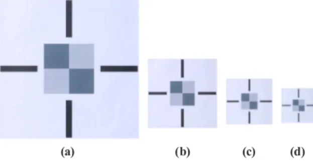
A set of four target sheets was used to measure the blur amount under varying FD and OD, which were utilized to observe edge displacements (Seo, 2017a; Seo, 2017b) and blurs (Seo, 2018a), Fig. 1 shows the design of the target sheets. Table 1 summarizes the dimensions of the parts shown in Fig. 1. The four elongated line regions were used to determine the reference lines of edges. The four square box regions were designed to generate edges occurring between their boundaries. Two of them located at upper left and lower right areas were designed to have relatively darker intensities.
In addition, the other two of them located at upper right and lower left areas were designed to have relatively brighter intensities. Four target sheets were designed to have different contrasts in the central box areas. Fig. 2 shows examples of the four target sheet images captured by a DSLR camera with OD = 2.0 m and FD = 2.0 m, thus which are images captured with a well-focused condition.
(a) (b) Fig. 1. Design of target sheets. (a) Annotation of target sheet dimensions; (b) Edge profile collection directions
Table 1. Target dimensions in Fig. 1(a) [mm]
Part a b c d
Length 9 52.5 35 9
(a) (b) (c) (d) Fig. 2. Images captured with OD = 2.0m and FD = 2.0m against varying contrasts. (a) Contrast-1; (b) Contrast-2;
(c) Contrast-3; (d) Contrast-4
2.2 Description of camera settings
Table 2 summarizes the specifications of the DSLR camera used in this study. The camera is a non-metric camera which is commonly available in the commercial camera market. As f-stop increases, the image becomes darker and edges are sharpend, approaching to a pin-hole image, while as f-stop decreases, the aperture size increases, which make the captured image become bright but edges in the image become blurred. Under the consideration of the influence of the f-stop on the image quality, the f-stop was set to f/8, which can be considered to be relatively large value when images are captured under indoor condition. To obtain images with suitable intensity values under relatively large f-stop, shutter speed was set to 1/2 s, which can be considered to be relatively large value compared to usual camera settings.
In order to acquire the target images with high fidelity, the sensitivity was set to ISO (International Organization of Standardization) 100, which is the smallest value provided by the camera, thus preventing large edge displacement due to contrast (Seo, 2017a; Seo, 2017b). The above settings of the camera were fixed to capture all the images for four target sheets during image acquisition.
2.3 Description of target image acquisition
For target image acquisition, FD of the camera was set to vary from 1.0 m-5.0 m with an interval of 0.5 m. For each setting of FD, images of the four target sheets were captured for varying OD from 1.0 m-5.0 m with an interval of 0.5 m.Table 2. Specifications of the DSLR camera used in this study
Category Characteristic Specification
Camera body
Model Nikon D300S
Image Sensor 23.6 mm × 15.8 mm CMOS sensor
Image size 4,288 × 2,848
File type TIFF
Lens Model Nikon AF NIKKOR 14 mm
Picture angle 90°
Camera settings
f-stop f/8
Shutter speed 1/2 s
Sensitivity ISO 100
Journal of the Korean Society of Surveying, Geodesy, Photogrammetry and Cartography, Vol. 38, No. 2, 109-121, 2020
Thereafter, a total of 324 images were captured for varying combination of FD, OD, and target sheet.
Fig. 3 illustrates the relationships among a camera lens, focal length, FD, target plane, OD, sensor plane, the CoC, and the diameter of CoC. FD indicates the distance between the lens and an object when the object is imaged sharply in the sensor plane. Target plane indicates the location where target sheets were placed. OD indicates the distance between the target plane and the lens. Under the assumption of the thin lens model, a point in the target plane is imaged into a point in the sensor plane, when OD is equal to FD. However, a real camera system does not map a point at FD to a point in the sensor plane because of a certain amount of blur caused by non-zero aperture and other factors of a lens system. This will be shown in the experiment section.
Fig. 3. Focal length (f), FD, OD, and the diameter of CoC (c) for a thin lens model
The diameter of the CoC of a lens c is calculated (Hecht, 2001; Zhuo and Sim, 2011) as
×
(1)
where f and N are the focal length and the f-stop number of the camera, respectively. In addition,
×
and
×
represent OD and FD, respectively which are shown in Fig. 3.
Fig. 4 shows the images captured for the target sheet Contrast-4 against varying OD under FD = 1.0 m. As shown in Fig. 4, the sharpest image was captured at OD = 1.0 m because OD = FD and image blur was shown to grow as the difference between OD and FD increased because of defocus blur.
(a) (b) (c) (d) Fig. 4. Images captured for Contrast-4 with FD = 1.0m against varying OD. (a) OD = 1.0 m; (b) OD = 2.0 m; (c)
OD = 3.0 m; (d) OD = 4.0 m
2.4 Estimation of blur function parameters
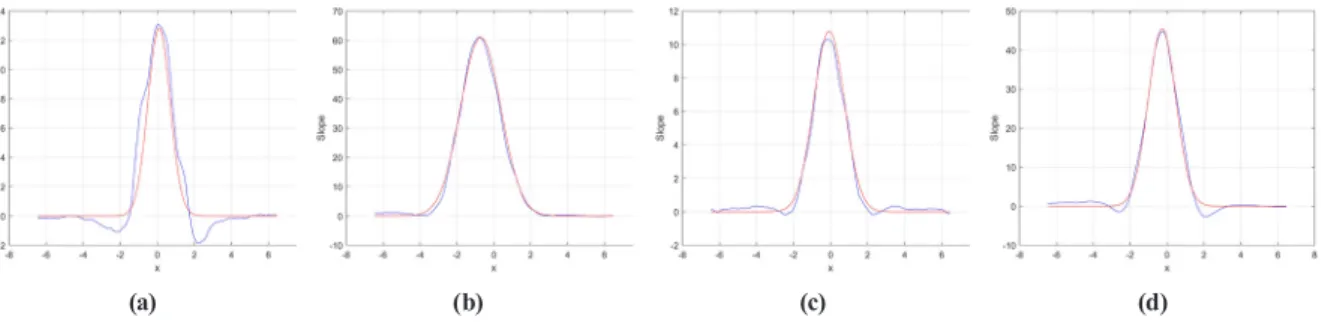
In this study, the blur function is modeled by the slope profiles of the intensity profiles of edges in the direction normal to the reference lines. Intensity values were collected, and then resampled with an interval of 0.1 pixels. Then, the mean value of intensities at each resampled location was calculated by finding the mean of all the intensity values at that location. Next, slope profiles were derived from resampled intensity values by differentiating them. In addition, the blur function is modeled by a one-dimensional Gaussian function which has one blur parameter. In reality, blurs occurring in camera imaging were shown to be modeled better by a function with two blur parameters than a function with one blur parameter (Seo, 2018a). But for the simplicity of blur parameter estimation, a Gaussian function with one blur parameter was used to model the blur function. Because of the difficulty to fit a Gaussian function to observed slope profiles, this study used the brute-force blur parameter estimation method described in Seo (2018a).Fig. 5 shows examples of the slope profiles and their fitted blur function for varying OD, FD, contrast, and color band. As shown in Fig. 5, the slope profiles can be modeled suitably by a Gaussian function with one blur parameter in many cases. However, Fig. 5(a) shows that the observed slope profiles have some lower values than the modeled value, which could be fitted well by two blur parameter model (Seo, 2018a) but this problem was disregarded in this study. Table 3 summarizes the specifications of the cases shown in Fig. 5.
σ and δ represent the blur and edge displacement parameters, respectively (Seo, 2017a; 2017b). As summarized in Table 3, the blur parameter became small when OD was close to FD and became large when OD was apart from FD. Edge displacement was shown to become large in the negative direction (from bright to dark regions) when contrast at edge grew. These effects will be investigated more comprehensively in the experiment section.
3. Experiments
3.1 Derivation of theoretical blurs
In order to compare the coincidence between the theoretical blurs and real blurs captured by a DSLR camera, theoretical blurs were first calculated according to Eq. (1). The variables in Eq. (1) were set to equal to their corresponding parameters in Table 2. F-stop of the camera
×
and focal length
×
were set to 8 and 14 mm, respectively. OD was set to vary from 1.0 m – 5.0 m with an interval of 1 mm. Because the pixel size of the camera
×
is 5.5 μm and
×
indicates the diameter of the CoC,
×
is divided by 2Χ0.0055 in order to find their corresponding blur amount in camera pixels.
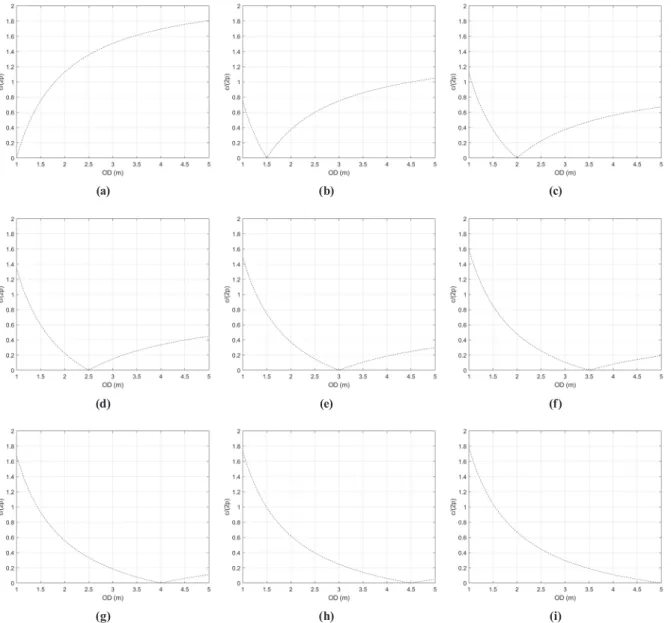
Fig. 6 shows the theoretical blur amount of a thin lens camera calculated under the condition of the camera settings used in this study. As shown in Fig. 6, the theoretical blur amount ranges from 0.0-1.8 pixels under the camera settings.
Fig. 5. Fitting results for slope profiles. Blue and red lines indicate the observed slope profiles and their fitted function, respectively
Table 3. Specifications and estimates of the slope profiles in Fig. 4
Case OD FD Target Band Estimates
σ δ
Fig. 5(a) 1.0 m 1.0 m Contrast-1 Red 0.60 0.10
Fig. 5(b) 1.0 m 5.0 m Contrast-2 Green 1.09 -0.71
Fig. 5(c) 2.0 m 3.0 m Contrast-3 Blue 0.83 -0.07
Fig. 5(d) 1.5 m 4.0 m Contrast-4 Red 0.75 -0.27
(a) (b) (c) (d)
Journal of the Korean Society of Surveying, Geodesy, Photogrammetry and Cartography, Vol. 38, No. 2, 109-121, 2020
3.2 Observed blurs
Fig. 7 shows the distribution of blurs observed in the four target images with different edge contrast against varying FD and OD. As shown in Fig. 7, the variation of blur was observed to be relatively large when FD is within 1.0 m-2.5 m. HoweveRi, the variation of blur was observed to be relatively small and the value of blur was observed to be relatively small when FD is greater than 2.5 m and OD is
greater than 2.0 m, which indicates that the camera was well- focused in the cases. The blurs occurring when FD = 1.5 m were observed to be smaller than the blurs when FD = 1.0 m and 2.0 m. This effect is considered to have been caused due to the internal mechanism of the DSLR camera, thus which is considered to be difficult to identify the cause exactly with the experiments performed in this study and to require a further investigation on the camera’s internal mechanism.
Fig. 6. Theoretical blur amount corresponding to the camera settings under the assumption of a thin lens camera. (a) FD = 1.0 m; (b) FD = 1.5 m; (c) FD = 2.0 m; (d) FD = 2.5 m; (e) FD = 3.0 m; (f) FD = 3.5 m; (g) FD = 4.0 m; (h) FD = 4.5 m; (i) FD
= 5.0 m;
(a)
(d)
(g)
(b)
(e)
(h)
(c)
(f)
(i)
(a)
(b)
(c)
(d)
Red Green Blue Fig. 7. Observed blurs
×
against FD and OD. (a) Contrast-1; (b) Contrast-2; (c) Contrast-3; (d) Contrast-4
Journal of the Korean Society of Surveying, Geodesy, Photogrammetry and Cartography, Vol. 38, No. 2, 109-121, 2020
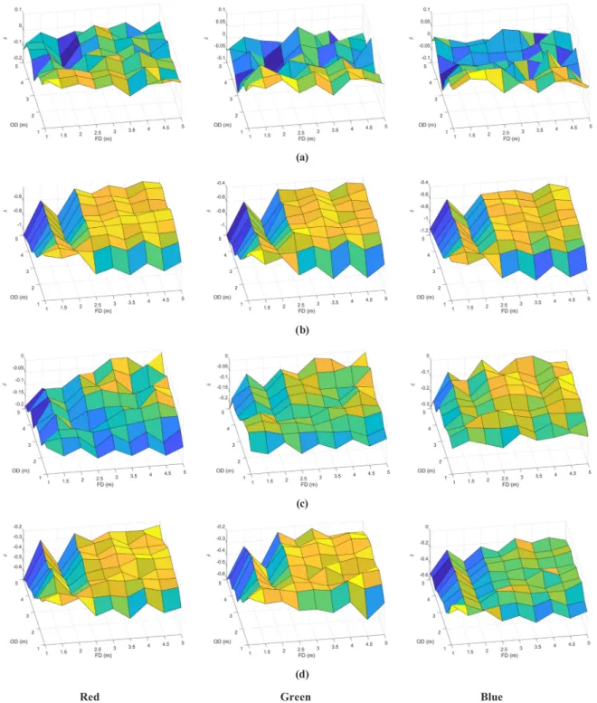
3.3 Observed edge displacements
Fig. 8 shows the distribution of edge displacement
×
of the four target images with different edge contrast under the
varying combination of FD and OD. As shown in Fig. 8, the magnitude of edge displacement was observed to increase when edge contrast increased.
(a)
(b)
(c)
(d)
Red Green Blue Fig. 8. Observed edge displacements
×
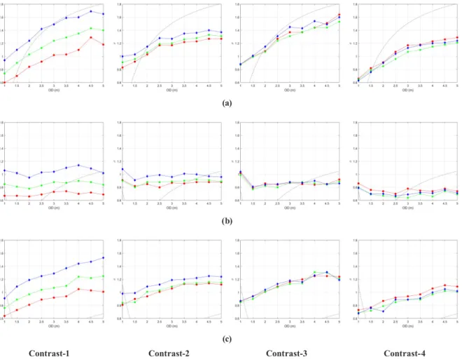
against FD and OD. (a) Contrast-1; (b) Contrast-2; (c) Contrast-3; (d) Contrast-43.4 Comparison of observed blurs with theoretical blurs
Fig. 9 shows the comparison of the blur variations of theoretical blur amount derived from a thin lens model according to Eq. (1) and the blurs observed in the images captured by the DSLR camera. As shown in Fig. 9, the discrepancy between the theoretical blur amount and the blur amount of the DSLR camera was found to be non-trivial. In addition, the pattern of the discrepancy was found to depend on color band, edge contrast, FD, and OD. As shown in Fig.
9(a), the blurs of the DSLR camera were smaller than their theoretical amount when FD = 1.0 m and OD was greater
than 2.0 except the blur band of Contrast-1. In addition, as shown in Fig. 9(b). the blurs of the DSLR camera were observed to be similar values across all tested ODs, which are largely apart from their corresponding theoretical values.
Fig. 9(c) also shows that the blurs of the DSLR camera were largely apart from their corresponding theoretical values.
However, the tendency of the nonlinear increase of blur when OD grew was observed in the blur variations when FD
= 1.0 m and FD = 2.0 m. This indicates that the usage of blur for depth calculation is partly possible for the specific combinations of edge contrast, color band, and FD.
(a)
(b)
(c)
Contrast-1 Contrast-2 Contrast-3 Contrast-4 Fig. 9. Observed blurs
×
against OD under given FDs. (a) FD = 1.0 m; (b) FD = 1.5 m; (c) FD = 2.0 m. Black dashed line represents the theoretical amount of blur for a thin lens camera. Red, green, blur lines represent the blur of red, blue, and
green bands, respectively
Journal of the Korean Society of Surveying, Geodesy, Photogrammetry and Cartography, Vol. 38, No. 2, 109-121, 2020
3.5 Tendency of observed edge displacements
Fig. 10 shows the pattern of variations of the edge displacement againt FD, OD, color band, and edge contrast. As shown in Fig. 10, the differences among the edge displacements of three color bands were observed to be trivial. Low contrast (Contrast-1 and Contrast-3) were observed to generate small magnitude of the edge displacement. Medium contrast (Contrast-4) and high contrast (Contrast-2) were observed to generate non-trivialamount of the edge displacement. In addition, the cases of Contrast-2 and Contrast-4 shows a certain trend of variation of edge displacement against OD. The trend indicates that the edge displacement increases in the negative direction as OD increase for the given FDs. This indicates that the edge displacement may be used to calculate object depth if measurement of the edge displacement is possible in an image.
(a)
(b)
(c)
Contrast-1 Contrast-2 Contrast-3 Contrast-4 Fig. 10. Observed edge displacements
×
against OD under given FDs. (a) FD = 1.0m; (b) FD = 1.5m; (c) FD = 2.0m. Red, green, blur lines represent the edge displacement of red, blue, and green bands, respectively3.6 Experiments with natural images
Experiments with natural images were performed to compare the variations of blurs in natural images with those in the target images. Fig. 11 shows the natural images captured with FD = 1.0 m, 1.5 m, and 2.0 m, respectively with the same settings of the camera as those used for capturing target images. The three FDs were only used because FDs greater than 2.0 m were observed to generate well-focused images in the experiments with the target images. In the natural images, seven edges shown in Fig. 11 were selected to extract edge profiles along them. The contrast of the edges selected in the natural images are similar to that of the target sheet Contrast-1. The distances of the edges from the camera were measured and regarded as ODs.
Edge profiles of the edges were accumulated and their centers were shifted to 0 location using the subpixel edge localization method described in Seo (2018b). Then, their mean and slope profiles were calculated. Next, the blur amount of each slope profile was estimated using the blur estimation method described in Seo (2018a).
Fig. 12 shows the blur variations observed in the natural images. In the followings, the results shown in Figs. 9 and 12 are compared. As shown in Fig. 12(a), when FD = 1.0 m, the blurs were observed to tend to increase when the difference between OD and FD increased but the pattern of their variations was found not to be matched exactly to that observed in the target sheet images. As shown in Fig.
12(b), when FD = 1.5 m, the blurs were observed to increase
(a)
Fig. 11. Natural images captured with different FDs. (a) FD = 1.0 m; (b) FD = 1.5 m; (c) FD = 2.0 m. Red lines indicates the locations of edges whose cross-section profiles were inspected
(b) (c)
(a)
Fig. 12. Observed blurs σ in natural images against OD under given FDs. (a) FD = 1.0 m; (b) FD = 1.5 m; (c) FD = 2.0 m.
Red, green, blur lines represent the blur of red, blue, and green bands, respectively
(b) (c)
Journal of the Korean Society of Surveying, Geodesy, Photogrammetry and Cartography, Vol. 38, No. 2, 109-121, 2020
when the difference between OD and FD increased but their variations were not matched exactly to the trend obtained from the target sheet images. As shown in Fig. 12(c), when FD = 2.0 m, the blurs were observed to be smaller than those observed in the target sheet images. Thus, from the experiments, we can consider that the blur variations of target images and natural images are not exactly matched but have a common effect that blurs tend to increase when the difference between FD and OD increases, which is observed distinctively when FD is relatively small, for example, FD = 1.0 m in the experiments.
4. Conclusion
This study investigated the pattern of the variations of edge blur against edge contrast, FD, and OD with a set of target sheet images and natural images obtained by a DSLR camera. The variations of edge blur amount observed under varying edge contrast, FD, and OD were compared with their theoretical blur amount derived from a thin lens model. The experimental results show that the observed edge blurs were significantly different from their corresponding theoretical amount. However, the experimental results show that the tendency of the increase of edge blur with the increase of difference between FD and OD was observed in most cases, which is distinct when FD is relatively small, for example, FD
= 1.0 m. In addition, edge displacement was also observed to have the tendency of the increase of the displacement magnitude for the edges with moderate to high contrast.
Thus, this study shows that the edge blur can be utilized to calculate the depth of objects from a single image for certain cases similar to the specific conditions shown to have the manifest tendency of the edge blur and the edge displacement between FD and OD in the experiments.
Acknowledgment
This research was supported by Basic Science Research Program through the National Research Foundation of Korea(NRF) funded by the Ministry of Education(2016R1 D1A1B02011625).
References
Cao, Y., Fang, S., and Wang, Z. (2013), Digital multi- focusing from a single photograph taken with an uncalibrated conventional camera, IEEE Transactions on Image Processing, Vol. 22, No. 9, pp. 3703-3714.
Chen, S.-J. and Shen, H.-L. (2015), Multispectral image out- of-focus deblurring using interchannel correlation, IEEE Transactions on Image Processing, Vol. 24, No. 11, pp.
4433-4445.
De, I., Chanda, B., and Chattopadhyay, B. (2006), Enhancing effective depth-of-field by image fusion using mathematical morphology, Image and Vision Computing, Vol. 24, pp. 1278-1287.
Gajjar, R. and Zaveri, T. (2017), Defocus blur parameter estimation using polynomial expression and signature based methods, 4th International Conference on Signal Processing and Integrated Networks, 2-3 February, Noida, India, pp. 71-75.
Green, P., Sun, W., Matusik, W., and Durand, F. (2007), Multi-aperture photography, ACM Transactions on Graphics, Vol. 26, No. 3, Article 68.
Hecht, E. (2001), Optics, 4th ed., Addison Wesley.
Hong, Y., Ren, G., Liu, E., and Sun J. (2015), A blur estimation and detection method for out-of-focus images, Multimedia Tools and Applications, Vol. 75, pp. 10807- 10822.
Karaali, A. and Jung, C.R. (2018), Edge-based defocus blur estimation with adaptive scale selection, IEEE Transactions on Image Processing, Vol. 27, No. 3, pp.
1126-1137.
Kim, S., Lee, E., Hayes, M.H., and Paik, J. (2012), Multifocusing and depth estimation using a color shift model-based computational camera, IEEE Transactions on Image Processing, Vol. 21, No. 9, pp. 4152-4166.
Lu. Q., Zhou, W. Fang L., and Li, H. (2016), Robust blur kernel estimation for license plate images from fast moving vehicles, IEEE Transactions on Image Processing, Vol. 25, No. 5, pp. 2311-2323.
Moghaddam, M.E. (2007), A mathematical model to estimate out of focus blur, 5th International Symposium on Image and Signal Processing and Analysis, 27-29
September, Istanbul, Turkey, pp. 278-281.
Oliveira, J.P., Figueiredo, M.A.T., and Bioucas-Dias, J.M.
(2014), Parametric blur estimation for blind restoration of natural images: linear motion and out-of-focus, IEEE Transactions on Image Processing, Vol. 23, No. 1, pp.
466-477.
Reuter, A., Seidel, H.-P., and Ihrke, I. (2012), BlurTags:
spatially varying PSF estimation with out-of-focus patterns, 20th International Conference on Computer Graphics, Visualization and Computer Vision, June, Plenz, Czech Republic, pp. 239-247.
Seo, S. (2017a), Prediction of edge displacement due to image contrast, The Photogrammetric Record, Vol. 32, No. 158, pp. 119-140.
Seo, S. (2017b), Estimation of edge displacement against brightness and camera-to-object distance, IET Image Processing, Vol. 11, No. 8, pp. 568-577.
Seo, S. (2018a), Edge modeling by two blur parameters in varying contrasts, IEEE Transactions on Image Processing, Vol. 27, No. 6, pp. 2701-2714.
Seo, S. (2018b), Subpixel edge localization based on adaptive weighting of gradients, IEEE Transactions on Image Processing, Vol. 27, No. 11, pp. 5501-5513.
Sun, T.-Y., Ciou, S.-J., Liu, C.-C., and Huo, C.-L. (2009), Out- of-focus blur estimation for blind image deconvolution:
using particle swarm optimization, Proceedings of the 2009 IEEE International Conference on Systems, Man, and Cybernetics, 11-14 October, San Antonio, Texas, pp.
1627-1632.
Tang, C., Hou, C., and Song, Z. (2013), Defocus map estimation from a single image via spectrum contrast, Optics Letters, Vol. 38, No. 10, pp. 1706-1708.
Wu, S. and Lin, W. (2008), Defocus estimation from a single image, Proceedings of 17th International Conference on Computer Communications and Networks, 3-7 August, St. Thomas, US Virgin Islands, pp. 1-5.
Yuan, L., Sun, J., Quan, L., and Shum, H.-Y. (2007), Image deblurring with blurred/noisy image pairs, SIGGRAPH-07: Special interest group on computer graphics and interactive techniques conference, August, San Diego, California, pp. 1-es.
Zhang, Y. and Hirakawa, K. (2015) Fast spatially varying object motion blur estimation, IEEE International Conference on Image Processing, 27-30 September, Quebec City, Canada, pp. 646-650.
Zhang, Y. and Hirakawa, K. (2016) Blind deblurring and denoising of images corrupted by unidirectional object motion blur and sensor noise, IEEE Transactions on Image Processing, Vol. 25, No. 9, pp. 4129-4144.
Zhou, C., Lin, S., and Nayar, S. (2009), Coded aperture pairs for depth from defocus, IEEE 12th International Conference on Computer Vision-2009, 29 September-2 October, Kyoto, Japan, pp. 325-332.
Zhu, X., Cohen, S., Schiller, S., and Milnafar, P. (2013), Estimating spatially varying defocus blur from a single image, IEEE Transactions on Image Processing, Vol. 22, No. 12, pp. 4879-4891.
Zhuo, S. and Sim, T. (2011), Defocus map estimation from a single image, Pattern Recognition, Vol. 44, pp. 1852- 1858.