Complexity Estimation Based Work Load Balancing for a Parallel Lidar Waveform Decomposition Algorithm

(1)

1. Introduction

LIDAR is an active remote sensing technology which provides 3D coordinates of the Earth’s surface

by performing range measurements from the sensor.

The range measurements are obtained by measuring the time difference between an outgoing signal and a return signal (which is also called a return waveform.)

Complexity Estimation Based Work Load Balancing for a Parallel Lidar Waveform Decomposition Algorithm

Jinha Jung*, Melba M. Crawford*, and Sanghoon Lee**^†

*Laboratory for Applications of Remote Sensing, Purdue University, West Lafayette, IN 47906

**Department of Industrial Engineering, Kyungwon University, Seongnam-shi, Kyunggi-do, Korea

Abstract : LIDAR (LIght Detection And Ranging) is an active remote sensing technology which provides 3D coordinates of the Earth’s surface by performing range measurements from the sensor. Early small footprint LIDAR systems recorded multiple discrete returns from the back-scattered energy. Recent advances in LIDAR hardware now make it possible to record full digital waveforms of the returned energy.

LIDAR waveform decomposition involves separating the return waveform into a mixture of components which are then used to characterize the original data. The most common statistical mixture model used for this process is the Gaussian mixture. Waveform decomposition plays an important role in LIDAR waveform processing, since the resulting components are expected to represent reflection surfaces within waveform footprints. Hence the decomposition results ultimately affect the interpretation of LIDAR waveform data.

Computational requirements in the waveform decomposition process result from two factors; (1) estimation of the number of components in a mixture and the resulting parameter estimates, which are inter-related and cannot be solved separately, and (2) parameter optimization does not have a closed form solution, and thus needs to be solved iteratively. The current state-of-the-art airborne LIDAR system acquires more than 50,000 waveforms per second, so decomposing the enormous number of waveforms is challenging using traditional single processor architecture. To tackle this issue, four parallel LIDAR waveform decomposition algorithms with different work load balancing schemes - (1) no weighting, (2) a decomposition results-based linear weighting, (3) a decomposition results-based squared weighting, and (4) a decomposition time-based linear weighting - were developed and tested with varying number of processors (8-256). The results were compared in terms of efficiency. Overall, the decomposition time-based linear weighting work load balancing approach yielded the best performance among four approaches.

Key Words :LIDAR,Waveform, Decomposition,Gaussian Mixture, Parallel Computation.

Received December 20, 2009; Revised December 24, 2009; Accepted December 26, 2009.

†Corresponding Author: Sanghoon Lee ([email protected])

(2)

Traditional small footprint LIDAR systems record multiple discrete returns from the back-scattered energy. These multiple returns are transformed into 3D coordinates in combination with the location (obtained from GPS (Global Positioning System)) and the attitude (obtained from the IMU (Inertial Measurement Unit)) of the sensor. Recent advances in LIDAR hardware now make it possible to record full digital waveforms of the returned energy. The full waveform LIDAR system has recently attracted attention of researchers because more information may be extracted from LIDAR waveform data than traditional LIDAR point cloud data.

The first LIDAR full waveform digitizer system was developed in the 1980s for bathymetric applications. Topographic full waveform profiling digitizer systems began to be marketed in the 1990s (Mallet and Bretar, 2009). More recently, the Laser Vegetation Imaging Sensor (LVIS) was developed as a prototype for the Vegetation Canopy LIDAR (VCL) mission. It is an airborne large footprint full waveform system and operates at altitudes up to 10 km while acquiring data in swaths up to 1,000 m with 25 m nominal waveform footprints. It has been acquiring data since 1997 (Blair et al., 1999). In addition to the airborne full waveform LIDAR system, the Ice, Cloud and Land Elevation Satellite (ICESat), a spaceborne large footprint full waveform LIDAR system, was launched in 2003 and operated until recently. The primary goal of this mission is to measure elevation changes in the arctic and the Antarctic to understand how changes in ice-sheet mass balance impact global sea level changes. In addition to this objective, the ICESat mission also enables precise measurement of land topography and provides information on vegetation structure by recording and processing the Geoscience Laser Altimeter System (GLAS) waveforms (Zwally, 2002). Other than NASA full waveform LIDAR

systems, the University of Texas at Austin developed an airborne small footprint full waveform LIDAR system by integrating a waveform digitizer developed by Optech, Inc. with the traditional multiple returns LIDAR system (Gutierrez et al., 2005). Commercial small footprint airborne full waveform scanning LIDAR systems also have been available since 2004 (Mallet and Bretar, 2009), although data have not typically been fully exploited in analysis.

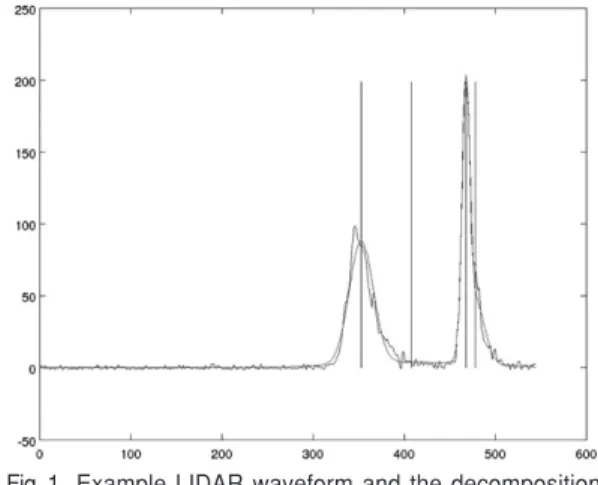
LIDAR waveform decomposition refers to the process of decomposing a return waveform into a mixture of components which are then used to characterize the original waveform data. The most common statistical mixture model used for the process is the Gaussian mixture, whose parameters include mixing coefficients and the mean and standard deviation of each component. Fig. 1 shows an example of LIDAR waveform and its decomposition results. A blue line is the received LIDAR waveform from the sensor, a red line is the estimated waveform from the decomposition results, and black line is the location of the estimated mean of the decomposed Gaussian components. Waveform decomposition plays an important role in LIDAR

Fig. 1. Example LIDAR waveform and the decomposition result (Blue line: the received LIDAR waveform, Red line: the estimated waveform from the decomposition result, Black line: the location of the estimated mean of Gaussian components).

(3)

waveform processing because the resulting decomposed components are assumed to represent reflection surfaces within waveform footprints.

Hence the decomposition results ultimately affect the interpretation of LIDAR waveform data. Various researchers utilized a Gaussian mixture model to decompose LIDAR waveform into components (Chauve et al., 2007; Hofton et al., 2000; Jung and Crawford, 2008; Persson et al., 2005). A LIDAR waveform decomposition algorithm proposed by Jung and Crawford (2008) is used in this study.

Most discrete return LIDAR systems not only use proprietary algorithm to detect peaks so the end-user has no way to assess the quality of the results, but also limits number of returns (usually from 2 to 5) from a waveform. However, full waveform LIDAR data provide the end-user raw data to extract more accurate and meaningful information. Researchers (Reitberger et al., 2008) reported that a much higher point density was achieved by decomposing waveforms than conventional discrete return LIDAR system and higher classification accuracy was achieved. Other researchers (Duong et al., 2008) reported better extraction of canopy and ground elevations using the ICESat waveforms even in forested areas.

Decomposing the waveform into a mixture of Gaussians involves two separate, but related, problems; (1) estimation of the number of components in a mixture, and (2) optimization of the parameters of the components. Various methods to estimate the number of components and parameters have been proposed. Hofton et al. computed second derivatives of a smoothed waveform to find inflection points, and used the inflection points to estimate an initial number of components in a mixture and the parameters of the components. They utilized the Levenberg-Marquardt optimization method to obtain parameter estimates (Hofton et al., 2000). Persson et

al. (2005) smoothed the waveform prior to estimating the initial number of components by locating local maxima points, and used the EM algorithm as a parameter optimization method. Chauve et al. (2007) utilized the zero crossing of first derivatives of the smoothed waveform to estimate the number of components and initial parameters, and nonlinear least squares optimization methods were used to obtain the corresponding parameter estimates (Chauve et al., 2007). Jung and Crawford (2008) proposed a sequential approach which identifies an initial component and sequentially adds components until the parameter estimates satisfy stopping criteria, and used combination of nonlinear least squares and the EM variant algorithm (greedy EM and sequential EM) as parameter optimization methods.

Computational requirements in the waveform decomposition process result from two factors; (1) estimation of the number of components in a mixture and the resulting parameter estimates are inter-related and cannot be solved separately, and (2) the parameter optimization problem does not have a closed form solution, and thus needs to be solved iteratively. The current state-of-the-art airborne LIDAR system acquires more than 50,000 waveforms per second (Mallet et al, 2009), so decomposing the enormous number of waveforms is challenging using traditional single processor architecture. Furthermore, there may be a situation in which LIDAR waveform data need to be processed near real-time.

Identifying portions of the work that can be performed concurrently and mapping the associated work onto multiple processors are critical steps in parallel algorithm design. In a parallel LIDAR waveform decomposition algorithm, the first is trivial because the decomposition results from one waveform do not affect the decomposition of other waveforms. Hence, computation associated with a

(4)

single waveform can be run concurrently without problems. However, the latter - also known as work load balancing - is critical in developing a parallel LIDAR waveform decomposition algorithm because it affects the overall performance of the algorithm. To tackle this issue, a parallel LIDAR waveform decomposition algorithm with four different work load balancing schemes - (1) no weighting (NW), (2) a decomposition results based linear weighting (DRLW), (3) a decomposition results based squared weighting (DRSW), and (4) a decomposition time based linear weighting (DTLW) - were designed and tested with varying number of processors (8 - 256) in this study.

2. Experimental data

1) LIDAR waveform data

The Freeman Ranch is a research site located near San Marcos, TX (USA) and managed by Texas State University. It contains a mixture of rangeland and woodlands. Topography is primarily low hills divided by small creeks, except with steep slopes along drainage channels. An Optech ALTM (Airborne Laser Terrain Mapper) 1225 small footprint LIDAR system with a full waveform digitizer, which is owned and managed by the University of Texas at Austin (UT), was flown over Freeman Ranch on 12 August 2005. The UT LIDAR laser system operates at 1064 nm with a pulse rate of 25 kHz. Its waveform sampling rate is 1 ns, which corresponds roughly to 15 cm in the vertical dimension. Five flight lines were acquired at an altitude of 650 - 720 m above ground level with a resulting footprint diameter of approximately 13 - 14 cm (Neuenschwander et al., 2008). About 21 million waveforms were acquired in five strips, but only data from 4th strip, which

contains 2,867,200 waveforms, were used in this study.

2) Computational platform

The Steele community cluster, which is managed by RCAC (Rosen Center for Advanced Computing) at Purdue University, was used for the study. It consists of 893 nodes and 7,144 processors. Each node has two quad-core processors and either 16 GB or 32 GB of memory. They are inter-connected by either Gigabit Ethernet or Infiniband. All nodes run Red Hat Enterprise Linux 4 and use PBSPro 9 for job management. The parallel LIDAR waveform decomposition algorithm was implemented in the C programming language using GSL (GNU Scientific Library) for the implementation of the nonlinear least squares algorithm and MPI (Message Passing Interface) library for communication among processors.

3. Methodology

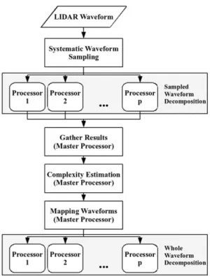
The proposed work load balancing for a parallel waveform decomposition algorithm is composed of two main steps; (1) complexity estimation, and (2) mapping waveforms onto multiple processors (Fig.

2). The NW approach does not perform complexity estimation and groups waveforms into subsets so that each subset contains the same number of waveforms.

The other three approaches (DRLW, DRSW, DTLW) perform complexity estimation and assign waveforms to subsets based on the estimated complexity. Here, complexity is estimated from the sampled waveforms. The computational requirements for decomposing a waveform into a mixture of Gaussian functions depends on the complexity of the waveform since it requires more time to decompose a waveform which contains more components than a

(5)

simple waveform. The three approaches other than the NW are designed to exploit the information on waveform complexity in order to balance work load among processors.

1) Decomposition of LIDAR waveform

A LIDAR waveform decomposition method proposed by Jung and Crawford (Jung and Crawford, 2008) is used in this study. It uses a Gaussian mixture model (Eq. 1) and sequentially decomposes a waveform into multiple components, where w(t) is the Gaussian mixture model, N is the number of components in a mixture, A_kis the amplitude, s_kis the standard deviation, and m_kis the mean of k_th component. For simple waveforms or well separated mixtures, a fast and simple non-linear least squares fit using Gauss Newton and the greedy EM algorithm are used, while, for more complex waveforms, the more robust EM and sequential EM methods are used

for the decomposition.

w(t) = A_k exp

[

^_

]

^{+ e} ⁽¹⁾

A region growing algorithm is used to estimate the initial parameters of each new component into the mixture. It uses the maximum value of the remaining waveform as the seed point to initiate the region growing process, and then terminates the region growing process when the value is smaller than a specified threshold value. Initial parameters are estimated from the grown region and input to one of the optimization methods.

An improvement (IMP) factor, which is based on SSE (Sum of Squared Error) value (Eq. 2), is defined to determine when to stop adding more components in a mixture (Eq. 3), where SSE_kis the SSE with k components, SSE₀is the SSE with no components, T is the length of the waveform in time (ns), w(t) is the received waveform, w_e,k(t) is the estimated waveform with k components, and IMP_kis the IMP value with k components.

SSE_k= (w(t) ^_w_e,k(t))² (2)

IMP_k= (3)

The IMP factor is used to determine whether the waveform approximation is adequate to justify terminating decomposition.

2) Complexity estimation

Three methods to estimate complexity of subsets, either from the decomposition results or the decomposition run time of the sampled waveforms, are proposed in this study. The DRLW and the DRSW approaches perform complexity estimation using the estimated number of components of the sampled waveforms, while the DTLW approach estimates complexity from the decomposition run

SSE₀^_SSE_k SSE₀

ST t=1

(t^_m_k)² 2s²_k 1

2ps²_k

SN k=1

Fig. 2. Flow chart of parallel waveform decomposition algorithm.

(6)

time of the sampled waveforms. Prior to complexity estimation, waveforms are first assigned to subsets with an equal number of waveforms, and a waveform is sampled from each subset. Waveforms are stored in time sequential order, so waveforms close to each other are expected to have similar shape and complexity. Therefore, the sampled waveforms are expected to represent the complexity of the subsets.

The same number of sampled waveforms from subsets are then distributed over processors, and decomposed into a mixture of Gaussians in parallel.

The decomposition results and decomposition run time of sampled waveforms from each processor are then gathered in a master processor so that the master processor can perform complexity estimation (Fig. 2).

The DRLW approach estimates the complexity of the subset (C_i) as the estimated number of components (n_i) of the sampled waveform (Eq. 4), and the DRSW approach estimates the complexity of the subset as the square of the estimated number of components of the sampled waveform (Eq. 5). The DTLW approach estimates the complexity of the subset as the decomposition run time (T_i) of the sampled waveform (Eq. 6).

C_i= n_i (4)

C_i= n²_i (5)

C_i= T_i (6)

3) Mapping waveforms onto multiple processors

For the NW approach, the master processor assigns temporally sequential waveforms to subsets so that each subset contains same number of waveforms. It does not utilize the results from the complexity calculations. For the other three approaches (DRLW, DRSW, DTLW), the master processor assigns waveforms to subsets so that each subset contains roughly the same complexity. In order to determine

the assignments of new subsets, the master processor finds the location where the estimated complexity exceeds ×100 (i = 1, ..., p^_1) percentile (p is the number of processors used in parallel execution and p_iis the processor number which is assigned to each processor from 0 to p ^_ 1). After the subsets assignments are made based on each work load balancing scheme, the subsets are distributed onto multiple processors for concurrent execution.

4. Results and discussion

The efficiency of parallel program is defined as the ratio between the speedup of parallel program (S) and the number of processors (p) used in parallel execution (Eq. 8), while the speedup of the parallel program is defined as the ratio between the best sequential algorithm run time (T_s) and parallel run time (T_p) (Eq. 7).

S = (7)

E = = (8)

A good parallel algorithm maintains its efficiency as the number of processors grows so that the number of processors may be scaled as the problem size grows (Grama, 2003).

Since the Steele community cluster is used by multiple users, the performance of the program may be affected by other users’ extensive usage of computational resources on the same node. The main goal of this study is to measure performance of work load balancing approaches, and it is critical to measure performance of the program accurately. In order to minimize the effect of the above phenomena, serial and parallel waveform decomposition algorithms are executed 20 times, and the best one

T_s pT_p S p

T_s T_p p_i

p

(7)

was selected to compute the efficiency. The best run time for serial waveform decomposition algorithm to decompose 2,867,200 waveforms was 8626 seconds (approximately 2 hours 24 minutes). Since the NW approach does not perform complexity estimation, the complexity estimation step was skipped and the same number of waveforms was distributed over processors for parallel execution. For the other three approaches, 1% of the waveforms were sampled systematically and the sampled waveforms were used to estimate the complexity measure for each subset.

After estimating complexity, waveforms were

divided into subsets according to the each work load balancing scheme, and the subsets were distributed over processors for parallel execution. Work load balancing approaches were tested on the Steele cluster using 8, 16, 32, 64, 128, and 256 processors.

Each approach was run 20 times, and the best one was selected to calculate the efficiency.

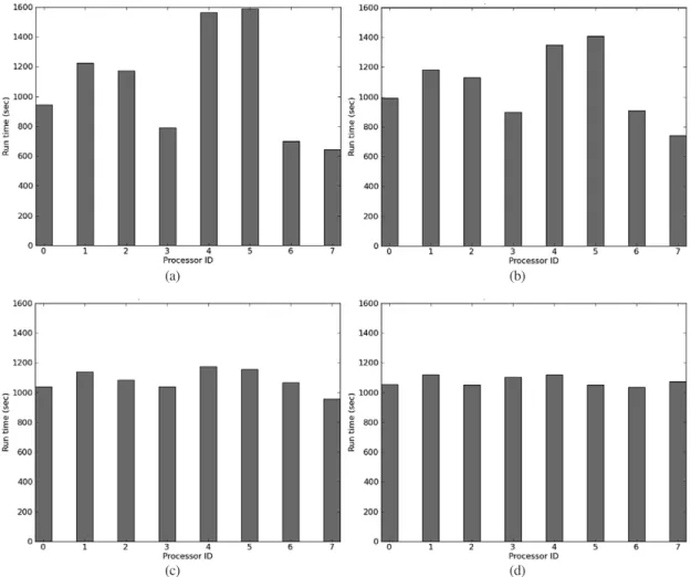
In each parallel execution, waveform decomposition run time for each processor was recorded. Fig. 3, 4, 5, 6 show the waveform decomposition run time of each work load balancing approach when 8, 16, 32, 64 processors are used for

Fig. 3. Waveform decomposition parallel run time of each processor when 8 processors are used with (a) no weighting (NW), (b) a decomposition results based linear weighting (DRLW), (c) a decomposition results based squared weighting (DRSW), and (d) a decomposition time based linear weighting (DTLW) work load balancing approaches.

(c) (a)

(d) (b)

(8)

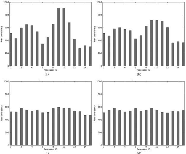
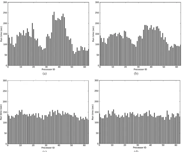
the parallel execution, respectively. These figures indicated that the NW approach showed the highest variance of decomposition run time among processors and the DRSW and the DTLW approaches showed the smallest variance. Smaller variance of decomposition run time implies better work load balancing among processors, since it indicates that fewer processors idle during the parallel execution.

Fig. 7 shows the resulting efficiency of four work load balancing approaches for a LIDAR waveform decomposition algorithm with varying number of

processors. Overall, the DTLW approach yielded the best efficiency, and the NW approach yields the worst efficiency. The DRSW approach was not as efficient, but showed similar performance as the DTLW approach. Fig. 7 also indicates that the efficiency decreases as the number of processors increases for all work load balancing approaches.

Work load balancing approaches based on the complexity estimation performed significantly better than the NW approach which does not perform complexity estimation.

(c) (a)

(d) (b)

(9)

5. Conclusion

Waveform decomposition is a critical process in LIDAR waveform data analysis, but requires extensive computation since estimation of the number of components and a parameter optimization process are inter-related, and parameter optimization must be done in an iterative manner. The current state-of-the- art airborne LIDAR system generates a massive volume of waveform data, and it is critical to process this volume of waveform data rapidly for some near real-time applications. To tackle this issue, four work

load balancing approaches for a parallel LIDAR waveform decomposition algorithm were proposed in this study. The work load balancing approaches were tested with varying number of processors and the results showed that the DTLW approach yielded the best performance and the NW approach yielded the worst performance among four approaches. Even though work load balancing approaches based on the complexity estimation showed better performance than the NW approach, the efficiency decreased as the number of processors increased for all work load balancing approaches. The best run out of 20 Fig. 5. Waveform decomposition parallel run time of each processor when 32 processors are used with (a) no weighting (NW), (b) a decomposition results based linear weighting (DRLW), (c) a decomposition results based squared weighting (DRSW), and (d) a decomposition time based linear weighting (DTLW) work load balancing approaches.

(c) (a)

(d) (b)

(10)

executions was used to compute efficiency of work load balancing approaches in this study. However, the worst execution is of concern in time critical applications, especially in an environment where multiple users share the same computational resources. A future study will investigate robustness of each work load balancing approach with larger number of processors.

(c) (a)

(d) (b)

Fig. 7. Efficiency of proposed work load balancing approaches (NW: No weighting, DRLW: Decomposition results based linear weighting, DRSW: Decomposition results based squared weighting, DTLW: Decomposition time based linear weighting).

(11)

Acknowledgment

This research was supported by a grant (07KLSGC03) from Cutting-edge Urban Development - Korean Land Spatialization Research Project funded by Ministry of Land, transport and Maritime Affairs of Korean government and by the Kyungwon University Research Fund in 2009.

References

Blair, J. B., Rabine, D. L, and Hofton, M. A., 1999, The Laser Vegetation Imaging Sensor: a medium- altitude, digitisation-only, airborne laser altimeter for mapping vegetation and topography. ISPRS Journal of Photogrammetry and Remote Sensing, 64: 115-122.

Chauve, A., Mallet, C., Bretar, F., Durrieu, S., Deseilligny, M.P., and Peuch, W., 2007, Processing full-waveform LIDAR data:

Modelling raw signals. ISPRS Workshop on Laser Scanning 2007 and SilviLaser 2007, pp. 102-107.

Duong, V. H., Lindenbergh, R., Pfeifer, N., and Vosselman, G., 2008, Single and two epoch analysis of ICESat full waveform data over forested areas. International Journal of Remote Sensing, 29(5): 1453-1473.

Grama, A., Gupta, A., Karypis, G., and Kumar, V., 2003, Introduction to parallel computing.

Addison-Wesley Longman Publishing Co., pp. 85-142.

Gutierrez, R., Neuenschwander, A., and Crawford, M. M., 2005, Development of Laser Waveform Digitization for Airborne LIDAR

Topographic Mapping Instrumentation.

Geoscience and Remote Sensing Symposium, 2005. IGARSS 2005. IEEE International, pp.

1154-1157.

Hofton, M. A., Blair, J. B., and Minster, J., 2000, Decomposition of Laser Altimeter Waveforms.

IEEE Transactions on Geoscience and Remote Sensing, 38(4): 1989-1996.

Jung, J. and Crawford, M. M., 2008, A Two-Stage Approach for Decomposition of ICESat Waveforms. Geoscience and Remote Sensing Symposium, 2008. IGARSS 2008. IEEE International, pp. 680-683.

Mallet, C. and Bretar, F., 2009. Full-waveform topographic lidar: State-of-the-art. ISPRS Journal of Photogrammetry and Remote Sensing, 64(1): 1-16.

Neuenschwaner, A. L., Urban, T. J., Gutierrez, R., and Schutz, B. E., 2008, Characterization of ICESat/GLAS waveforms over terrestrial ecosystems: Implications for vegetation mapping. 2008, American Geophysical Union, 113.

Persson, A., Soderman, U., Topel, J., and Ahlberg, S., Visualization and analysis of full-waveform airborne laser scanner data. ISPRS Workshop on Laser scanning 2005, pp. 103-108.

Reitberger, J., Krzystek, Pl, and Stilla, U., 2008, Analysis of full waveform LIDAR data for the classification of decisuous and coniferous trees, International Journal of Remote Sensing, 29(5): 1407-1431.

Zwally, H. J., 2002, ICESat’s laser measurement of polar ice, atmosphere, ocean, and land.

Journal of Geodynamics, 34: 405-445.