Implicit Surface Representation of Three-Dimensional Face from Kinect Sensor

Implicit Surface Representation of

Three-Dimensional Face from Kinect Sensor

수료 아드히 워보워* ․ 김은경* ․ 김성신**

Suryo Adhi Wibowo, Eun-Kyeong Kim, and Sungshin Kim

*부산대학교 전자전기컴퓨터공학과, **부산대학교 전기컴퓨터공학부

*Department of Electrical and Computer Engineering, Pusan National University

**School of Electrical and Computer Engineering, Pusan National University

본 논문은 BK21플러스, IT기반 융합산업 창 의인력양성사업단에 의하여 지원되었으며, 산업통상자원부가 지원하는 산업융합ㆍ연 계형 로봇창의인재양성사업의 연구결과로 수행되었음.(N0001126)

This is an Open-Access article distributed un- der the terms of the Creative Commons Attribution Non-Commercial License ( ht t p: / / c r ea t i v ec ommon s . or g / l i- censes/by-nc/3.0) which permits unrestricted non-commercial use, distribution, and re- production in any medium, provided the orig- inal work is properly cited.

Abstract

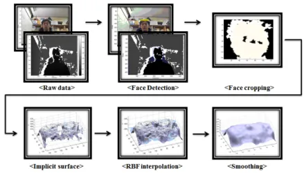
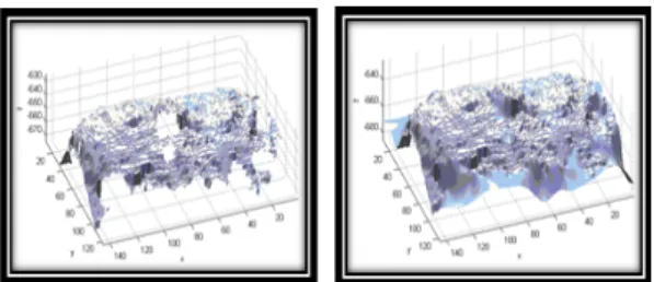
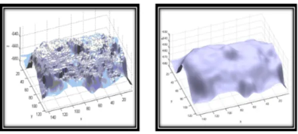
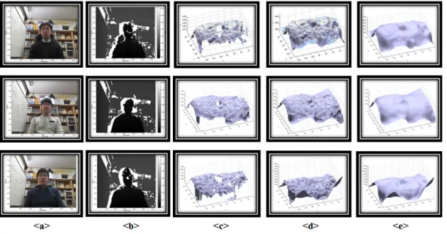
Kinect sensor has two output data which are produced from red green blue (RGB) sensor and depth sensor, it is called color image and depth map, respectively. Although this device’s prices are cheapest than the oth- er devices for three-dimensional (3D) reconstruction, we need extra work for reconstruct a smooth 3D data and also have semantic meaning. It happened because the depth map, which has been produced from depth sensor usually have a coarse and empty value. Consequently, it can be make artifact and holes on the surface, when we reconstruct it to 3D directly. In this paper, we present a method for solving this prob- lem by using implicit surface representation. The key idea for represent implicit surface is by using radial basis function (RBF) and to avoid the trivial solution that the implicit function is zero everywhere, we need to defined on-surface point and off-surface point. Based on our simulation results using captured face as an input, we can produce smooth 3D face and fill the holes on the 3D face surface, since RBF is good for in- terpolation and holes filling. Modified anisotropic diffusion is used to produced smoothed surface.

Key Words : Implicit surface, Radial basis function, Three-dimensional face, Kinect sensor.

Received: Mar. 22, 2015 Revised : Apr. 5, 2015 Accepted: May. 5, 2015

†Corresponding author [email protected]

1. Introduction

In this decades, electronic devices which has relation with graphics such as smart- phone, television, 3D scanner and other device has been growth rapidly. We also known that the printer device has been development to the 3D printer. This condition contributes to the research on computer graphics field which is also growth rapidly.

We could make an avatar for virtual reality games or we could make a model which is represent our self and then we can print it using 3D printer, where this work has been performed[1]. In computer graphics area, this research called surface re- construction and reconstruct a surfaces that have semantic meaning results are a chal- lenge for researcher.

Surface reconstruction could be more difficult if the device for data acquisition pro- duces noisy data and many holes. This condition will be happen if we used the cheapest device for 3D data acquisition like Kinect sensor. Kinect sensor can capture 30 images per second and this device has specification range for the depth, which is between 1.2m to 3.5m. Kinect sensor could produce many holes when we take the depth map data f rom the distance less than 1.2m. Although we captured the depth map in the spesification range, the raw data that we get are still contain a lot of noise. The holes could be filled by using some methods such as volumetric diffusion, neighborhood method, or interpolation method likes RBF interpolation.

At the first time RBF was introduced by Powell, he provided an algorithm with a re- start procedure that takes account of the objective function automatically [2].

Broomhead and Lowe have done the development from Powell’s researchthe relation-

ship between learning in adaptive layered networks and the fitting of data with high

Fig. 1. Framework.

dimensional surfaces [3]. Surface interpolation for medical imaging using RBF method is proposed [4].

RBF is also has been proposed f or interpolating im- plicit surface from scattered surface data [5]. In this paper we present 3D face representation using RBF and Kinect sensor with the distance is less than 1.2m.

This research makes the following contributions:

1. Providing a f illing holes method f or the 3D surface 2. Providing a smoothing method for 3D surface The organization of this paper is as follows. Section 1 introduces surface reconstruction and previous research us- ing RBF interpolation. In Section 2, data acquisition and preprocessing are presented in detail. In Section 3, we de- scribe the implicit surface. Section 4 introduces smoothing of 3D surface. Section 5 presents the experiments and results. Finally, we present our conclusions in Section 6.

2. Data acquisition and preprocessing

Our framework shown on figure 1 which have data ac- quisition step, preprocessing step, implicit surface, and smoothing step. In this section, we describe about data acquisition and preprocessing step in detail.

2.1 Data acquisition

Assume a person sit in f ront of the device f or data acquisition. We used the kinect sensor as a device for da- ta acquisition. It produces good depth map data when the distance between the person and the sensor are in the range 1.2–3.5m but in our system, we used the distance less than 1.2m.

We capture the RGB image and depth map from the person one time. The size of the RGB image and depth

map are same. We used 480×640 as the size of the RGB image and depth map which is represent rows and col- umn of image, respectively. The RGB image consist three channels (red, green, and blue channel) which have 8 bits in each channel or equal to 0-255 for represent a color.

Depth map consist 11 bits which is represent the distance between the object to the kinect. This values represent on millimeter.

2.2 Preprocessing

We have two raw data, the RGB image and depth map. Because the focus of this research is about the face, so we need determined the position of the face. Because of this reason, we need algorithm for face detection. Face detection will be implement on the RGB image, it is caused the RGB image has an information more useful than depth map.

Viola and Jones [6] has been finished outstanding result of their research. They made an algorithm for detection the face. In their research, they made three contribution.

First contribution is integral image. Integral image is image representation which allows the features used by their de- tector to be computed very quickly. Second contribution is simple and efficient classifiers. They used AdaBoost learn- ing algorithm for selecting a small number of critical visual feature from very large set of potential feature. The last contribution is a method for combining classifiers in a

“cascade” which allows background regions of the im- age to be quickly discarded while spending more compu- tation on promising face-like regions. Because of this rea- son, we used viola-jones face detection in our research.

We used this method to RGB image.

After we determined face position and region from RGB

image, we should determined face position and region

from depth map. Since we did not perform camera cali- bration before, we could not alignment between face posi- tion and region from RGB image to depth map directly.

We should extend the box size which is represent face position and region from the output of face detection.

Then we can crop the depth map.

The cropped depth map that obtained from the pre- vious step is not only contains face, background or the other object are also included in this image. To eliminate this problem, we perform some preprocessing step. First, we compute minimum value from cropped depth map.

This value represent the nose, where nose is the object that has nearest distance with kinect sensor. The second step is estimate the distance range of the face. We ob- served this distance range and we conclude that the dis- tance which represent the face are between minimum val- ue of cropped depth map to 50mm f urther away. Since the smallest value resulting from the depth map will high- ly affect in the 3D reconstruction, even though zero value, so we implement not a number in the third step. Not a number will be represent not face, and it will be combine to the previous step. The last step is generate point cloud from previous step that it represents geometry. This point cloud represented as  ,where  represent cartesian coordinate and  is represent the value from depth map which has correlation with .

3. Implicit surface

In this section, we present implicit surface representation. Following Carr et al [7], implicit surface representation is made by using RBF. Briefly, implicit sur- face representation is an approach to model the surface implicitly with a function .If a surface consist of all the points and satisfy the equation   , it could be said that  implicitly def ines the surf ace. Two important things in this step are constructing signed-distance function and fitting an RBF to the resulting distance function.

3.1 Fitting an implicit function to a surface

The problem in this section is how to find a function  which implicitly defines a surface and satisfies the equa- tion   . This result will be zeros in all of points because points  will be lying on the surface. To avoid this condition, we should add some point called off-sur- face point and are given non-zero value.

The new problem is how to generate the off-surface point and what is the value will be corresponding to the

off-surface point. Following [7] the off-surface point will be given positive sign if that point is on outside of the surface, and will be given negative sign if that point is on the inside of the surface. Off-surface point could be gen- erate by calculate surface normals. In the other word, off-surface point is the surface normals. Now we have on-surface points which is represent surface points and off-surface points which is represent surface normals. By using on-surface points and off-surface points, we could find the implicit function using approach for interpolation problem.

3.2 Radial basis function interpolation

The set of on-surface points and off-surface points that we have is the kind of a scattered data. For the inter- polation problem, it is scattered data interpolation problem. To solve this problem, we approach with to used RBF. RBF f unction could be determined as follow:

   _{  }  ^{          (1)}

where  is a polynomial low degree and the basic function  is a real valued function on ∞.The points

  are represented as a center of the RBF and  is equal to the number of points .

The existing basic function  that often to use in the RBF are the gaussian (usually used in the neural network), thin-plate spline (usually for smoothing and need input two variable), multiquadric, biharmonic (Eq. 1), and triharmonic. In this research we used biharmonic basic function because we want to fit with three variables which represent the coordinate of the points . Eq. 1 could be formulated as a linear system, and this linear system can be written as follows, and where  is the value of surface normal and  is polynomial coefficient.

After we determined the RBF interpolant, we can fit this interpolant to the surface which is generate based on grid representation, and the range of value  on grid rep- resentation are from minimum to the max-

Fig. 2. 3D face before (left) and after (right) interpolation using

RBF.

Fig. 4. (Left) Ground truth data, (Center) example of preforated surface and (Right) result of RBF interpolation.

Fig. 3. 3D face before (left) and after (right) smoothing using modified anisotropic diffusion.



  ^{ } ⋮ ⋮ ⋱ ⋮ ⋮ ⋮ ⋮ ⋮ ^{      ⋯  ⋯                   } 

    ⋯         

  ⋯     

    ⋯      

    ⋯      

    ⋯      



  ^{ ⋮               }  ^{     ⋮             (2)}

imum value of each other. We can get new values of  by using this procedure. Figure 2 shown the result of the interpolation using RBF. In this example, we used  is equal to 26994.

4. Smoothing

Since the result from interpolation using RBF still coarse, we will perform smoothing in this step in order to get smooth surface. Suryo and co-worker [8] perform smoothing surface using modified anisotropic diffusion. In their work, the detect not a number (nan) and replace this value to the zero while perf orm anisotropic diffusion.

We follow their work for our smoothing process.

Begin with the result from interpolation using RBF, we have the new points data about  ,we called this as    _  _  _   _   _ , and   consist of 2D array, respectively. Because of

 _   _  represent value from mesh grid data and it is important to constructing triangle mesh, so we did not

set this value as an input to smoothing process using modified anisotropic diffusion. The input for modified ani- sotropic diffusion that we set are only from   values.

So, the input for modified anisotropic diffusion are 2D array.

This smoothing process begin with calculating finite dif- ferences of each neighborhood pixel, this process need a 2D matrix mask with the size is 3×3 for each matrix. By using this matrix, calculating finite differences could be determined by performing convolution between   and 2D matrix. 2D matrix shown in Eq. 3



 

  ^

 

  

   

   

 

  ^

 

  

   

   

 

  ^

 

  

   

   



 

  ^

 

  

   

   

 

  ^

 

  

   

   

 

  ^

 

  

   

   



 

  ^

 

  

   

   

 

  ^

 

  

   

   

(3)

Eq. 4 shown about the convolution between 2D matrix mask and 

,



 





 





 







 





 





 







 





 



(4)

 is the convolution result.

After this we determined the convolution result, the next step for smoothing process is calculating partial dif- ferential equation by using Eq. 5,

     ∙ _{  }  ^{ }

   ^{    }  ^{ ∙   (5)}

where    is equal to 0.2 and  is equal to 10.

The last step for smoothing process are replace nan

with the zero in the , after this we can determined

Fig. 5. <a> is raw data of RGB image, <b> is raw data of depth map, <c> is 3D face contains holes and coarse surface,

<d> is the result of RBF interpolation, and <e> is smoothing resu lt u sing modified anisotropic diffusion.

new value from   by using Eq. 6.

    _   (6)

this process (Eq. 4 to Eq. 6) will be repeated until the number of iterations. In this example, the number of iterations that we used is 10 iterations. Figure 3 shown the comparison of 3D face before smoothing and after smoothing.

5. Experiment

In our experiment, we used three different people and each person has four different data. All the data contains many holes and noisy. By using the data, we perform testing procedure to determine the performance of our algorithm. We can see that holes in the 3D face could be filled by using RBF. By performing RBF and modified ani- sotropic diffusion, we can get smooth surface and also the holes could be filled.

Since we did not have ground truth data, we could not know the performance of RBF interpolation. In this section, we will calculate the perf ormance of RBF inter- polation using RMSE. The ground truth data generated based on our simulation and artificial holes will be em-

bedded in to the ground truth data, it will become new data called perforated surface. This perforated surface will

be set to be the input of RBF interpolation, and we will calculate the RMSE between the result of RBF interpolation and the ground truth data. Figure 4 illustrated the ground truth data, example of preforated surface and the result of RBF interpolation.

RMSE calculated from 5 preforated surfaces with differ- ent number of holes. Table 1 shows the result of RMSE.

Based on Table 1, RBF interpolation can be used to fill the hole and this method produces little error. The exam- ple result of the testing process is illustrated in the right- most of Figure 4.

Name Number of holes RMSE

Preforated_surface_1 1 0.00056

Preforated_surface_2 2 0.00081

Preforated_surface_3 3 0.00053

Preforated_surface_4 4 0.00051

Preforated_surface_5 5 0.00055

Preforated_surface_6 6 0.00022

Preforated_surface_7 7 0.00014

Preforated_surface_8 8 0.0003

Preforated_surface_9 9 0.00024

Preforated_surface_10 10 0.00024

Table 1. Result of RMSE from preforated surface

6. Conclusions

This paper presents a method to filled the holes and produces smooth result with the single input data (single RGB and single depth map). For fill the holes, we should determined about implicit surface, and this problem could be solved by using RBF interpolation, since this problem is kind of scattered data problem.

For avoid trivial solution problem which is zero every- where, signed-distance function should be determined.

Modified anisotropic diffusion can be used to produce smooth surface. Based on the simulation to produce smooth surface. Based on the simulation from artificial da- ta, RBF is one of robust method for scattered data inter- polation problem.

References

[1] H. Li, E. Vouga, A. Gudym, L. Luo, J. T. Barron, and G. Gusev, “3D Self-Portraits,” ACM Transaction on Graphics, vol. 32, no. 6, pp. 187, 2013,

[2] M. J. D. Powell, “Restart Procedures for The Conjugate Gradient Method,” Mathematical

Programming, vol. 12, no. 1, pp. 241-254, 1977.

[3] D. S. Broomhead and D. Lowe, “Multivariable Functional Interpolation and Adaptive Network,”

Complex System, vol. 2, no. 3, pp. 321-355, 1988.

[4] J. C. Carr, W. R. Fright, and R. K. Beatson.,

“Surface Interpolation with Radial Basis Function f or Medical Imaging,” IEEE Transaction on Medical Imaging, vol. 16, no. 1, pp. 96-107, 1997.

[5] B. S. Morse, T. S. Yoo, D. T. Chen, and K. R.

Subramanian, “Interpolating Implicit Surfaces from Scaterred Surface Data Using Compactly Supported Radial Basis Functions” in Proceeding of International Conference on Shape Modelling and Applications, pp. 89-98, Genova, 2012.

[6] P. Viola and M. J. Jones, “Robust Real-Time Face Detection,” International Journal of Computer Vision, vol. 57, no. 2, pp. 137-154, 2004.

[7] J. C. Carr, R. K. Beatson, J. B. Cherrie, T. J.

Mitchell, W. R. Fright, B. C. McCallum, and T. R.

Evans, “Reconstruction and Representation of 3D Objects with Radial Basis Functions” in Proceedings 28th Annual Conference on Computer Graphics and Interactive Techniques, pp. 67-76, 2001.

[8] S.A. Wibowo and S. Kim, “Three-Dimensional Face Point Cloud Smoothing Based on Modified Anisotropic Diffusion Method,” International Journal of Fuzzy Logic and Intelligent Systems, vol. 14, no.

2, pp. 84-90, 2014.

저 자 소 개

수료 아드히 위보워(Suryo Adhi Wibowo) 2009년 : Telkom Institute of Technology

전기공학과 공학사

2012년 : Telkom Institute of Technology 전기공학과 공학석사

2014년~현재 : 부산대학교 전자전기컴퓨터 공학과 박사과정

관심분야 : Image Processing, Intelligent System Phone : +82-51-510-2367

E-mail : [email protected]

김은경(Eun Kyeong Kim) 2014년 : 부산대학교 전자전기공학부

공학사

2013년~현재 : 부산대학교 전자전기컴퓨터 공학과 석사과정

관심분야 : Intelligent system, Data mining Phone : +82-10-2888-5348

E-mail : [email protected]

김성신(Sungshin Kim) 1986년: 연세대학교 전기공학과

공학석사

1996년 : Georgia Inst. of Technology, 전 기및컴퓨터공학부 공학박사 1998년~현재: 부산대학교 전기컴퓨터공학

부 교수

관심분야 : Intelligent system, Intelligent robot, Fault diag- nosis and prediction

Phone : +82-51-510-2374

E-mail : [email protected]