1. Introduction
Researchers have turned to dynamical systems theory in studying transition to turbulence and this helped in gaining a fresh perspective in understanding the phenomenon. In dynamical systems theory, the presence of coherent structures in turbulent flow may be seen as low-dimensional invariant sets in phase space[4]. These coherent structures, which are spatiotemporally organized, appear when a turbulent state visits the neighborhood of such an invariant set for a substantial fraction of time.
The Navier-Stokes equation, which governs turbulent motion of viscous fluids, is an example of an infinite- dimensional dynamical system which may be approximately reduced to finite dimension[4]. In this equation, the simplest invariant solution can be an equilibrium or a time-periodic one. Researchers have searched for invariant solutions and analyzed numerically the long-term behavior on their stable and unstable manifolds. The computation of stable and unstable manifolds in state space is relevant in the study of the transition process.
In wall-bounded shear flows, where laminar state is often linearly stable during transition to turbulence, an invariant set with only a single unstable direction in phase
space is called an ‘edge state’[10]. The edge state has a special property in which its stable manifold separates the laminar and turbulent flows. State points on this laminar- turbulent boundary, known as the ‘edge of chaos’[1,10], is attracted to the edge state. For initial conditions just exceeding a critical value, corresponding state points will escape out of the laminar basin along the unstable manifold of the edge state.
We study a periodic edge state to the incompressible Navier-Stokes equation in plane Couette flow. It is shown that computation of its unstable manifold leads to several orbits which return to the edge state along its stable manifold. This suggests the formation of a homoclinic connection, i.e., the intersection of the unstable and stable manifolds for the same saddle-type invariant solution. Two of the homoclinic orbits found move closer to each other for decreasing Reynolds until they eventually collide.
2. Transitional Plane Couette Flow
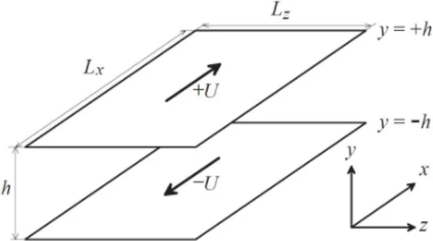
Shown above is the flow configuration of plane Couette flow that is employed in this study. This is composed of two parallel flat plates that are separated by a distance 2h.
The wall-parallel directions are the streamwise x- and spanwise z- directions while the wall-normal direction is the y- direction. The parallel plates move with the same velocity in the direction opposite each other, i.e., the upper plate is moving with velocity +U and the lower plate is moving with velocity -U.
The velocity field u = (u,v,w) for an incompressible viscous flow is governed by the Navier-Stokes equation Received: July 14, 2015, Revised: October 29, 2015,
Accepted: October 29, 2015.
* Corresponding author, E-mail: [email protected] DOI http://dx.doi.org/10.6112/kscfe.2015.20.4.058
Ⓒ KSCFE 2015
H OMOCLINIC O RBITS IN T RANSITIONAL P LANE C OUETTE F LOW
Julius Rhoan T. Lustro,*1 Genta Kawahara,2 Lennaert van Veen3 and Masaki Shimizu2
1College of Engineering and Agro-Industrial Technology, University of the Philippines Los Baños
2Graduate School of Engineering Science, Osaka University
3Faculty of Science, University of Ontario Institute of Technology
Recent studies on wall-bounded shear flow have emphasized the significance of the stable manifold of simple nonlinear invariant solutions to the Navier-Stokes equation in the formation of the boundary between the laminar and turbulent regions in state space. In this paper we present newly discovered homoclinic orbits of the Kawahara and Kida(2001) periodic solution in plane Couette flow. We show that as the Reynolds number decreases a pair of homoclinic orbits move closer to each other until they disappear to exhibit homoclinic tangency.
Key Words : subcritical transition to turbulence, periodic orbit, homoclinic orbit
Fig. 1 Plane Couette flow configuration
and continuity equation. The Reynolds number (Re) is written as Re = Uh/ν, where ν is the kinematic viscosity.
The nondimensionalized Navier-Stokes equation and continuity equation are given as
∙ ∇ ∇
∇ (1)
∇ ∙ (2)
The boundary condition of the flow is set to no-slip condition on the surface of the wall.
We consider Couette turbulence under similar conditions as those investigated by Hamilton et. al.[2]. Under this minimal plane Couette conditions, coherent structures in the near-wall region exhibit a regeneration cycle, which consists of formation and breakdown of streamwise vortices and low-velocity streaks. These streaks and vortices display complex behavior in both space and time.
The cyclic dynamics of the regeneration process in near-wall turbulence is the mechanism that sustains these coherent structures.
We perform direct numerical simulation of the incompressible Navier-Stokes equation for plane Couette turbulence by using a spectral method. The time-advancement is done by using 2nd-order Adam-Bashforth method for the nonlinear terms and Crank-Nicolson method for the viscous terms. The nonlinear time-periodic solution is obtained by using Newton-Krylov iteration(see [3] and [5]). The flow is supposed to have periodic boundary condition in the wall-parallel x and z directions. The computational periods are Lx = 1.755πh for the streamwise direction and Lz = 1.2πh for the spanwise direction. The dealiased Fourier expansions are employed in the wall-parallel directions and Chebyshev-polynomial expansion in the wall-normal
direction. Numerical computations are carried out on a resolution of 32 x 33 x 32 number of grid points in the streamwise, wall-normal, and spanwise directions, respectively. The number of degrees of freedom of the discretized system of the Navier-Stokes equation is N = 11,117. The spatial symmetries of Couette turbulence are observed without imposition in the flow. These two are as follows: reflection with respect to the plane of z = 0 accompanied by half period Lx/2 streamwise shift, and 180o rotation along the line x = y = 0 accompanied by half period Lz/2 spanwise shift. The shift-reflect and shift-rotate spatial symmetries are written as
The frictional force caused by the moving walls injects energy, where it is consumed at small scales over the whole flow field by viscous dissipation. The input (I) and dissipation (D) energy rates, both normalized with respect to their laminar state values, are given as
∣
∣
(3)
(4)where in (3) is the streamwise velocity and in (4) is the vorticity vector. The laminar state is represented by input and dissipation energy rates whose temporal average is equal to 1, while the turbulent state has input and dissipation energy rates whose temporal average is greater than 1. The gentle unstable periodic orbit (UPO)[3,5] lies in between the laminar and turbulent regions.
The UPO considered in this paper has only one unstable direction and thus it is an edge state. This UPO might be the only edge state in this computational domain.
For longer streamwise period, another edge state the Nagata’s lower-branch steady solution[7,9] appears. This UPO and its stable manifold can form the boundary separating laminar and turbulent flows.
3. Orbit Continuation
The UPO is extended by performing an orbit
continuation algorithm[8,11]. Consider an N-dimensional dynamical system
(5)
where ∈ represents a state point in an N-dimensional state space and ∈ represents the vector field obtained from the Navier-Stokes equation.
The orbitis given by the integration of equation (5) at any time . The initial condition is set as
(6)
where is some point on the UPO, is the unstable
2 3 4
2 3 4 5
I D
Fig. 3 Homoclinic orbits of the UPO at Re = 400 which are computed using single-shooting continuation. The two red orbits represent the same homoclinic orbits found by van Veen and Kawahara. The black orbit represents the new homoclinic orbit found in the present study
eigenvector at , and is a small parameter. We integrate (5) and monitor the behavior of the system by observing some physical quantities with time. In this paper we observe the values of the input and dissipation energy rates that are given in (3) and (4), respectively.
4. Homoclinic Orbits and Tangency
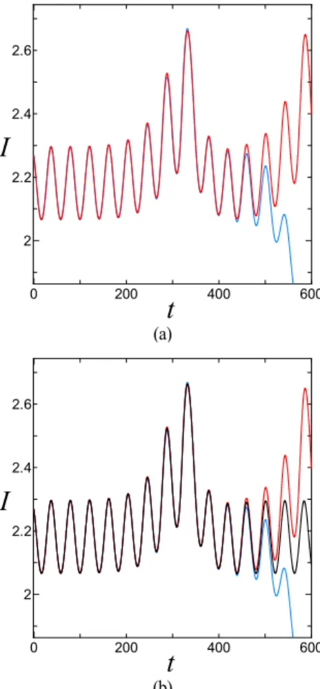
At the beginning a state point close to the UPO goes around its orbit for some time until it eventually escapes along the unstable manifold. As it is extended along the unstable direction, we observe that the orbit briefly return to the vicinity of the UPO along its stable manifold, then either relaminarize or swing up to turbulent region depending on the value of the parameter . The return of a state point to the UPO suggests a homoclinic connection.
To extract the homoclinic orbit, we select two values of that are near to each other with one relaminarizing after the brief return to the UPO (blue orbit in Fig.
2(a),(b) and the other going turbulent (red orbit in Fig.
2(a),(b)). Bisection is repeatedly applied in between these two values of until the period of the UPO after the return persists for a longer time (black orbit in Fig. 2(b)), i.e, the orbit loops back to the UPO for a number of times.
0 200 400 600
2 2.2 2.4 2.6
I
t
(a)
(a)
0 200 400 600
2 2.2 2.4 2.6
I
t
(b)
(b)
Fig. 2 (a) Orbit of two values of (red and blue lines) that will be used for bisection, (b) homoclinic orbit(black line) as a consequence of repeated bisection in between the two values of
2 2.5 2
3
I D
(a)
2 2.5
2 3
I D
(b)
(a) Re = 260 (b) Re = 250
2 2.5
2 3
I D
(c)
2 2.5
2 3
I D
(d)
(c) Re = 245 (d) Re = 241.3
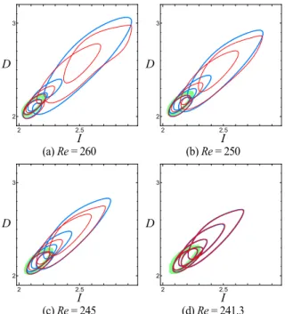
Fig. 4 A pair of homoclinic orbits projected on two-dimensional I-D plane for decreasing Reynolds number. The blue orbit is the smaller homoclinic orbit by van Veen and Kawahara while the red orbit is a newly discovered homoclinic orbit.
The light green orbit is the UPO
At Re = 400, van Veen and Kawahara[12] had found the existence of two distinct homoclinic orbits of the Kawahara and Kida gentle UPO using multiple-shooting orbit continuation[11]. These two homoclinic orbits are obtained again using the method described in the previous section, which can be called as single-shooting orbit continuation.
Results show that the homoclinic orbits previously obtained using multiple-shooting orbit continuation by van Veen and Kawahara are quantitatively and qualitatively similar to the ones we obtained using single-shooting orbit continuation(compare the red orbits in Fig. 3 with the orbits in [11]). Further computations reveal that another homoclinic orbit of the UPO is present at Re = 400. This new homoclinic orbit is shown in Fig. 3.
We proceed to tracking down homoclinic orbits to Reynolds numbers below Re = 400. Several homoclinic orbits are discovered and we find a pair of homoclinic orbits moving closer to each other for decreasing Reynolds number (see Fig. 4). One of the homoclinic orbits of the pair is the smaller homoclinic orbit by van Veen and Kawahara and the other is one of the newly discovered homoclinic orbits. The pair move closer until they overlap
with each other and become one. We call the Reynolds number where the pair overlap as tangency Reynolds number (ReT). We observe that ReT = 241.3. Below this Reynolds number, we do not find homoclinic orbits.
5. Summary
We investigated a time-periodic solution to the Navier-Stokes equation and found the existence of homoclinic orbits of this edge state. The discovery of several homoclinic orbits aside from the previously reported ones confirms the existence of infinitely many UPOs. As such, turbulence in shear flows can be seen as something that is governed by chaotic attractors, which reproduces the regeneration cycle[3].
We observed, qualitatively and quantitatively, a pair of homoclinic orbits moving closer to each other for decreasing Reynolds number. These orbits then collided at a tangency Reynolds number ReT = 241.3. The tangency Reynolds number suggests the Reynolds number where the appearance of homoclinic orbits happens.
The appearance of homoclinic orbits that was presented here adds another element in the elucidation of turbulence in terms of dynamical systems theory. It is important in the future that homoclinic orbits, as well as other connecting orbits of invariant sets that might be present, be investigated further in relation to turbulence in shear flows.
Acknowledgement
J.R.T.L. was supported by OVCRE Basic Research Program and Academic Development Fund of University of the Philippines Los Baños, and UP Research Dissemination Grant.
References
[1] 2008, Eckhardt, B., Faisst, H., Schmiegel, A. and Schneider, T.M., "Dynamical systems and the transition to turbulence in linearly stable shear flows,"
Phil. Trans. R. Soc. A, 366:1297-1315.
[2] 1995, Hamilton, J.M., Kim, J. and Waleffe, F.,
"Regeneration mechanisms of near-wall turbulence structures," J. Fluid Mech., 287:317-348.
[3] 2001, Kawahara, G. and Kida, S., "Periodic motion embedded in plane Couette turbulence: regeneration
cycle and burst," J. Fluid Mech., 449:291-300.
[4] 2012, Kawahara, G., Uhlmann, M. and van Veen, L.,
"The significance of simple invariant solutions in turbulent flows," Annu. Rev. Fluid Mech., 44:203-25.
[5] 2005, Kawahara, G., "Laminarization of minimal plane Couette flow: going beyond the basin of attraction of turbulence," Phys. Fluids, 17:041702.
[6] 1987, Kim, J., Moin, P. and Moser, R., "Turbulence statistics in fully developed channel flow at low Reynolds number," J. Fluid Mech., 177:133-166.
[7] 2005, Jimenez, J, Kawahara, G., Simens, M.P. et. al.,
"Characterization of near-wall turbulence in terms of equilibrium and ‘bursting’ solutions," Phys. Fluids, 17:01510.
[8] 2013, Lustro, J.R.T., van Veen, L. and Kawahara, G.,
"Long-term rigorous numerical integration of Navier-Stokes equation by Newton-GMRES iteration,"
TNUAA, Vol.30, No.3:248-251.
[9] 1990, Nagata, M., "Three-dimensional finite-amplitude solutions in plane Couette flow: bifurcation from infinity," J. Fluid Mech., 217:519-527.
[10] 2006, Skufca, J., Yorke, J. and Eckhardt, B., "The edge of chaos in a parallel shear flow," Phys Rev.
Lett., 96:174101.
[11] 2011, van Veen, L., Kawahara, G. and Matsumura, A., "On matrix-free computation of 2d unstable manifolds," SIAM J. Sci. Comput., 33:25-44.
[12] 2011, van Veen, L. and Kawahara, G., "Homoclinic tangle on the edge of shear turbulence," Phys Rev.
Lett., 107:114501.