OCEAN COLOR IMAGER
Jung-Hoon Kim,*1 Hyoung Yoll Jun,1 Cho Young Han1 and Byoungsoo Kim2
정지위성 해색 촬영기의 열모델링 기술
김 정 훈,*1 전 형 열,1 한 조 영,1 김 병 수2
Conductive and radiative thermal model configurations of an imager of a geostationary satellite are presented. A two-plane method is introduced for three dimensional conductive coupling which is not able to be treated by thin shell plate thermal modeling technique. Especially the two-plane method is applied to massive matters and PIP(Payload Interface Plate) in the imager model. Some massive matters in the thermal model are modified by adequate correction factors or equivalent thickness in order to obtain the numerical results of thermal modeling to be consistent with the analytic model. More detailed nodal breakdown is specially employed to the object which has the rapid temperature gradient expected by a rule of thumb. This detailed thermal model of the imager is supposed to be used for analyses and test predictions, and be correlated with the thermal vacuum test results before final in-flight predictions.
Key Words : Thermal Modeling, Two-lane Method, Interface Conductance, FEM, FDM, GOCI, COMS
Received: April 22, 2010, Revised: June 22, 2010, Accepted: June 25, 2010
1 Satellite Thermal & Propulsion Dpt., KARI, Daejeon 305-333, Republic of Korea
2 Department of Aerospace Engineering , Chungnam National Univiversity, Daejeon 305-764, Republic of Korea
* Corresponding author, E-mail: [email protected]
1. INTRODUCTION
This paper discusses the details of thermal model of the GOCI(Geostationary Ocean Color Imager) main unit which is installed in COMS(Communication, Ocean, and Meteorological Satellite) of Korea[1]. GOCI is known as the first ocean color imager operated on the geostationary orbit. Conductive and radiative configurations of the GOCI thermal model are presented in this paper. Since 1960's, thin shell plate modeling have been prefered in the spacecraft thermal engineering because of its heritage and well-established numerical and/or experimental database[2].
Therefore, the basic method for thermal modeling recalls the two-dimensional thin shell plate modeling technique.
Hereafter, a newly devised two-plane method is introduced for three dimensional conductive coupling adapted to the general thin shell plate thermal modeling. Some massive matters in the thermal model are modified by adequate correction factors or equivalent thicknesses in order to obtain the numerical results of thermal modeling to be consistent with the analytic model. More detailed nodal breakdown is specially employed to the FPA(Focal Plane Array), PIP(Payload Interface Plate) bipods, entrance baffle, pupil and the pointing mirror of the GOCI[3].
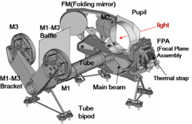
Thermica v3.2[4] is used as building up the thermal models by using the thin shell plates thermal meshing. As a result, the mathematical thermal model of GOCI includes 3674 lumped capacity nodes[5]. The GOCI element names used in this paper are given in the Fig. 1 and Fig. 2. GOCI is extensively composed of the telescope, FPA, mechanisms, and secondary structure enveloping the former elements. In order to analyze the accurate thermal behavior of GOCI, detailed radiative and
Fig. 2 GOCI Telescope
Fig. 1 Overview of GOCI without radiators and MLI
Fig. 3 Heat capacity difference between the analytic and numerical model
Fig. 4 Conductive coupling difference between the analytic and numerical model
conductive thermal models representative of the physical characteristics are necessary.
2. THERMAL MODELING OF MIRRORS
2.1GENERAL
Thin shell plates are used in thermal modeling for all mirrors.
The two-dimensional heat conduction can be only considered when thin shell plates are all used up in the thermal model. All the face sides of thin shell plates are both active in thermal radiation except for the mounting feet which are modeled in as non-active radiative surfaces on their contact area. Masks are included in the model when necessary. All the optical faces of the mirrors are modeled with triangular thermal nodes in order to avoid the surface warping which would be appeared in quadrangle thermal nodes. At least two thermal nodes in the height (axial direction) are modeled for all stiffeners in order to get the axial temperature gradient of the mirrors. The conductive coupling calculation is formed by
using FEM method. Edge nodes are used to simulate the conductive heat transfer and are not included in the other sub-models except in the main thermal model.
2.2 THERMAL MODEL THICKNESS CORRECTION
Most of the mirror components are based on thin shell plate modeling, however, for massive matters such as a mast which connects the mounting feet and the optical face are exception to this fact. The mirrors are divided into several components. For example, the components includes the outer/radial/circumferential stiffeners (inner and outer); lower/middle/upper mast, mounting feet, and the optical face. Sometimes high thicknesses, for example, more than 0.01 m induce the overestimation and/or underestimation in heat capacity and conductive coupling calculation for curved shapes. In Fig. 3 and Fig. 4, the differences are illustrated between the analytic model and the numerical model when the models are divided into six nodes. The thick solid line is a numerical thin shell plate edge in the geometrical model, and the dashed line is the
Component
Heat capacity Conductive coupling Analytic
(J/K)
Numerical (J/K)
Correction factor
Analytic (W/K)
Numerical (W/K)
Correction factor Lower mast 49.654 63.581 0.781 5.500 4.296 1.280 Middle mast 10.387 16.257 0.639 1.719 1.098 1.565 Table 1 Numerical correction factor in heat capacity and
conductive coupling
Mirror Description Thickness before correction(m)
Thickness after correction(m) Note
Pointing mirror
Outer stiffener 0.002 0.002
Radial stiffener 0.0015 0.0015 Circum.(Inner)
stiffener 0.0015 0.0015
Circum.(Outer)
stiffener 0.0015 0.0015
Lower mast 0.016 0.0205 1)
Middle mast 0.012 0.0188 1)
Upper mast 0.003 0.003
Feet 0.005 0.005
Optical face 0.0022 0.0022
1) Thicknesses are not acceptable in thin shell plate modeling for cylindrical shapes. Correction is inevitable.
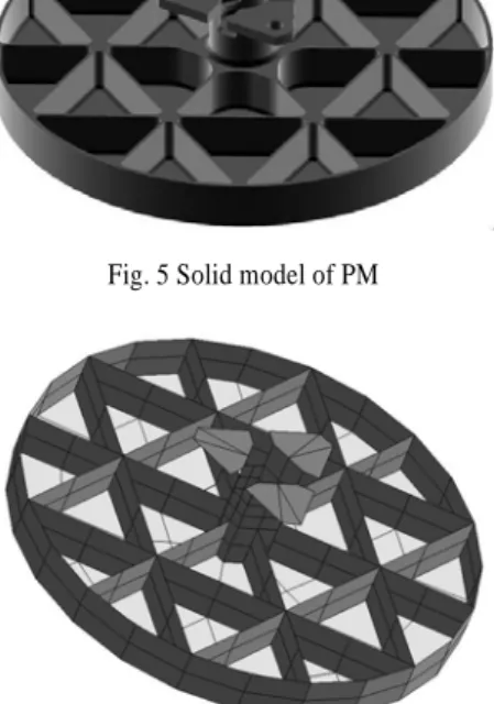
Table 2 Correction of each component thicknesses Fig. 5 Solid model of PM
Fig. 6 Thermal model of PM
volume of each thin shell plate. The heat capacity of numerical model is generally larger than the analytic model because the thickness of the numerical model is constant with radius direction by thin shell plate modeling.
Therefore, some additional volumes should be included in heat capacity calculation. On the other hand, in the numerical model, the conductive thermal path length between adjacent nodes is longer than the analytic model, which concludes that the conductance of the nodes are the smaller ones. Numerical correction factors which are equivalent to the results from the analytic model are obtained in the calculation of heat capacity and conductive coupling.
In M1, M3, FM and PM mirrors thermal modeling, there are lower and/or middle mast components having high thicknesses with curved shapes. It is necessary to check if there is any compatibility between the analytic calculation and the numerical calculation. The numerical radiative area is always shown as the flat surface in thin shell plate modeling, which is smaller than the analytic one since the numerical radiative area is unable to take over the real outer curved shape into consideration. These radiative area corrections are not considered in this modeling.
the pointing mirror is shown in Fig. 6. The radiative thermal model is exactly used as shown in Fig. 6.
However each quadrangle, rectangle, or triangle node has different thicknesses corresponding to the solid model illustrated in Fig. 5. There are two components, lower and middle mast that should be considered by correction factors in the pointing mirror thermal modeling. The calculation results for the heat capacity and conductive coupling correction of the mirror are shown in Table 1 accompanying their correction factors. The thickness correction made for each component of the mirror is shown in Table 2.
2.4 M2 MIRROR MODELING AND TWO-PLANE METHOD The solid model of the GOCI M2 mirror is shown in Fig. 7. The mirror material that is used is also SiC.
Three-dimensional conduction heat transfer simulation is impossible to function in the thin shell plate thermal
Solid shape Numerical control volume
Characteristicthicknessofthenodes
Conductive coupling using FEM
Manual conductive coupling using local analysis
Solid shape Numerical control volume
Characteristicthicknessofthenodes
Conductive coupling using FEM
Manual conductive coupling using local analysis
Fig. 8 Schematic of two-plane method
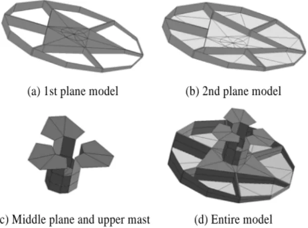
(a) 1st plane model (b) 2nd plane model
(c) Middle plane and upper mast (d) Entire model Fig. 9 Conductive thermal model configurations of M2 mirror Fig. 7 Solid model of the M2 mirror
model which is made in Thermica ver. 3.2. Therefore, a new method is developed that enables the simulation of the three-dimensional conduction heat transfer using a thin shell plate thermal model and which is called “Two-plane method”. The two-plane method uses:
― Two thin shell plate thermal mesh
― Each thin shell plate mesh has the conductive coupling inside its internal mesh(using FEM / local analysis)
― The third direction of heat path between the two thin shell plate meshes is modeled by using the local analysis method(GL=kA/L)
The case when the thin shell plate mesh has a variable cross-sectional area along to the heat path, the characteristic thicknesses of the thin shell plate mesh are determined by choosing the arithmetic average thickness of the minimum and maximum thicknesses for a given mesh.
The schematic that describes the two-plane method is shown in Fig. 8. For the M2 mirror, total three massive matters are considered as in the three-dimensional heat conduction simulation. Two massive matters are generated from each of the half of the outer stiffener and the
massive triangle which supports the optical face.
Another massive matter is called the middle mast which connects the massive triangle to the mounting feet. These three massive matters are represented by a thin shell plate that contains high thickness. Each thin shell plate is thermally coupled by the conductive conductance manually.
The M2 mirror thermal model configurations are shown in Fig. 9(a-d). In these figures, the three thin shell plates representing massive matters and the heat capacity model of the M2 mirror are described. The conductive couplings of each of the planes are automatically calculated by FEM method in Thermica and the local analysis method is manually used in order to make conductive couplings between the planes. All sides of the wall of the radial stiffeners and the massive triangle that are not involved in the conductive model have the thickness of zero which is applicable only to the radiative geometry model. The M2 mirror thermal model configurations are shown in Fig.
9.(a) ~ Fig. 9.(d).
3. THERMAL MODELING OF FPA
The FPA(Focal Plane Array) of GOCI consists of the following components: detector, detector window, detector package, PCB, flexible leads, radiation shield, thermal shunt, radiator, FPA MLI(Multi-Layer Insultation), FPA bracket and a baffle. For conductive coupling calculation, it is essential for the the local analysis method to use the rectangular shape nodes. In otherwise the FEM analysis method that uses the edge nodes are used for the complex meshes of the nodes such as triangle or quadrangle nodes.
Thin shell plates which ignores their heat conduction along the thickness direction are used in the FPA thermal
Fig. 10 Radiative configuration of FPA
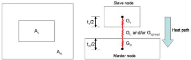
Fig. 11 Schematic of interface conductance
Fig. 12 Schematic of spreading conductance concept
Fig. 13 Conductive couplings in the PIP thermal model modeling, For every component different configuration is
used to make its conductive model. Then interface conductances are modeled to consider the contact heat transfer between these configurations. The calculation method of these interface conductances is described in more detail in section 3.1. The thermal shunts which are anticipated to have high temperature gradient are splited into five thermal nodes. Fig. 10 shows the radiative model of FPA.
3.1 INTERFACE CONDUCTANCE CALCULATION METHOD Each component of the FPA is linked by gluing and/or screwing the parts of the other component. In this case, an interface model is necessary to connect one component to the other one. The interface conductance between two components is generally determined by the serial thermal conductance circuit theory. Considering the two nodes which are in contact with each other; one node named as
"master node" and the other node named as "slave node"
for convenience’s sake. Once the thermal path through the interface surface is determined, the length of thermal path and the surface area normal to the path can be determined. The schematic for the interface conductance is
illustrated in Fig. 11. This method is useful when the contact areas of the nodes are not identical between adjacent two nodes which have a physical contact. The internal conductance of a slave node itself is[6]
(1)
where is the thermal conductivity of the slave node,
is the surface area normal to the heat path, and is the thickness of the slave node. For the same way the internal conductance of a master node itself is
(2)
where the subscription of means the master node.
Either using the gluing or screwing for the contact method, the contact conductance can be represented by
(3)
Fig. 14 Location of inserts considered in the PIP thermal model
Fig. 15 Overall thermal model of PIP
Fig. 16 Integrated GOCI model internal(without MLI covering)
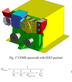
Fig. 17 COMS spacecraft with GOCI payload where is the surface conductance(W/m2K) and is
the contact area.
3.2 SPREADING CONDUCTANCE
Spreading effect on the contact area should be considered if the slave node consists some heat dissipation itself. The case does not only consider the power dissipation of slave node is greater than other amounts(depending on configurations) but also consider that the contact area() is lower than . If there is a contact area() dissipating heat on the master node area(), the represented temperature of the master node can be assumed as the temperature at the arithmetic average area between and . When the spreading conductance is ignored the temperature of the master node will be equaled to . The spreading conductance can be expressed by a non-linear formula as shwon below, and refer in Fig. 12 for the concept.
ln
(4)
The total conductance between nodes at the interface is defined by:
(5)
4. THERMAL MODELING OF PIP
For the conductive model of the PIP, two thin shell plate layers are considered; upper and lower PIP nodes.
The conductive couplings for each layer of the PIP nodes are calculated by the FEM coupling calculation module of Thermica (see Fig. 13). However the couplings between upper and lower layer of the PIP are calculated by the local analysis method manually(two-plane method).
It is necessary to consider the inserts in the heat capacity budget(when inserts are heavy);. Some inserts are considered at its location, other inserts’ capacities are spreaded on the all PIP area(on both layers of the PIP).
― For the telescope bipods interface : 6 interfaces on the PIP
― For the POM support interface : 3 interfaces on the PIP
― For the PIP bipods : 8 interfaces on the PIP
Fig. 14 shows the upper layer nodes of the PIP and corresponding massive inserts considered in the heat capacity model. These additional heat capacities of locally massive inserts are added to the corresponding PIP nodes.
The overall configuration of PIP and its bipods is shown in Fig. 15.
5. CONCATENATED GOCIMODEL
The details of integrated GOCI thermal model is shown in Fig. 16. In Fig. 17, the COMS spacecraft installing GOCI payload is illustrated along with other payloads in order to take into account the radiative environment by the external spacecraft geometry influencing GOCI thermal behavior.
6. CONCLUDING REMARK
Detailed thermal modeling has been performed for an
correction factor is contributed to compensate the volume loss resulted from sparse numerical meshing. This detailed thermal model of the imager is supposed to be used for analyses and test predictions, and be correlated with the thermal vacuum test results before final in-flight predictions.
REFERENCES
[1] 2008, Yang, K.H. et al., COMS System and Bus Development Project(V), Annual Report, KARI, Daejeon.
[2] 1986, Agrawl, B.N., Design of Geosynchronous Spacecraft, Prentice-Hall Inc., Washinton D.C.
[3] 2008, Kim, J.H., Description of GOCI Detailed Thermal Model, COMS document: COMS.DDD.
00048.DP.T.ASTR., EADS Astrium, Toulouse.
[4] 2003, Jacquiqau, M. and Noel, P., Thermica v3.2 User's Manual, EADS Astrium, Toulouse.
[5] 2008, Kim, J.H., GOCI Detailed Model Thermal Analysis, COMS document: COMS.TN.
00431.DP.T.ASTR., EADS Astrium, Toulouse.
[6] 2002, Gilmore, D.G., Spacecraft Thermal Control Handbook, AIAA Inc., Reston.