Information-Based Hybrid Modeling Framework on the Systematic use of Artificial Neural-Networks

Information-Based Hybrid Modeling Framework on the Systematic use of Artificial Neural-Networks

김 준 희† Jamshid Ghaboussi*

Kim, JunHee Jamshid Ghaboussi

···

요 지

본 논문에서는 수학적 구조 모델과 인공신경망 기법을 상호 유기적으로 결합하여 구조물의 거동 데이터로부터 부재모델 또는 재료모델의 정확도를 높이는 정보기반 하이브리드 모델 업데이트 기법을 개발하였다. 유한요소와 같은 수학적 모델을 사용하여 구조물의 거동을 모사하기 위해서는 재료, 부재, 그리고 시스템의 정확한 모델링이 우선하여야 한다. 그러나 재 료, 부재의 각 레벨에서의 수학적인 모델은 이상화과정을 거치면서 중요한 특성을 생략하거나, 시스템 구성시 부재간의 상 호작용이나 경계조건의 단순화로 인해 유한요소 모델은 실제 구조물의 거동과 차이를 보이게 된다. 본 논문에서 제시된 하 이브리드 모델 업데이트 기법은 구조물의 거동과 수학적 모델의 해석결과 차이를 인공신경망 기법을 사용하여 보완함으로 써 시스템 모델의 정확도를 높일 수 있다. 이때 시스템의 거동 데이터로부터 부재 또는 재료모델을 개선할 수 있는 데이터 를 추출하여 부재 또는 재료모델을 개선한다. 제시된 기법은 보-기둥 접합부의 이력모델을 개선하는 것으로 검증하였으며, 복잡한 거동을 보이는 시스템 모델링에 광범위하게 사용될 수 있다.

핵심용어 : 하이브리드 모델링, 모델 업데이트, 인공신경망, 정보기반 모델링, autoprogressive algorithm

Abstract

In this study, a new information-based hybrid modeling framework is proposed. In the hybrid framework, a conventional mathematical model is complemented by the informational methods. The basic premise of the proposed hybrid methodology is that not all features of system response are amenable to mathematical modeling, hence considering informational alternatives. This may be because (i) the underlying theory is not available or not sufficiently developed, or (ii) the existing theory is too complex and therefore not suitable for modeling within building frame analysis. The role of informational methods is to model aspects that the mathematical model leaves out. Autoprogressive algorithm and self-learning simulation extract the missing aspects from a system response. In a hybrid framework, experimental data is an integral part of modeling, rather than being used strictly for validation processes. The potential of the hybrid methodology is illustrated through modeling complex hysteretic behavior of beam-to-column connections.

Keywords : hybrid modeling, model update, artificial neural-networks, informational modeling, autoprogressive algorithm

···

†책임저자, 정회원, 한국건설기술연구원 수석연구원 Tel: 031-910-0230 ; Fax: 031-9100-392 E-mail: [email protected]

* University of Illinois at Urbana-Champaign, Professor Emeritus

∙이 논문에 대한 토론을 2012년 10월 30일까지 본 학회에 보내주 시면 2012년 12월호에 그 결과를 게재하겠습니다.

1. Introduction

The field of mechanics is concerned with the behavior of physical bodies subjected to external stimuli. A new data set is generated and collected

from a physical event. The information contained in the data set is then conveyed to a proper mathe- matical model, which is capable of representing that specific event or other similar events. The mathe- matical models have normally been accepted as the

Biologicallyinspired

Informational modeling approach

Conventional modeling approach Problem modeling

MathematicallyMathematicallybasedbased

Biologicallyinspired

Informational modeling approach

Conventional modeling approach Problem modeling

MathematicallyMathematicallybasedbased

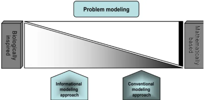
Fig. 1 Classification of modeling process

2. Mathematical modeling versus informational modeling

Modeling processes may be classified as mathe- matically based approaches and biologically inspired approaches, as can be seen in Fig. 1. A modeling process would be determined by how much a priori knowledge is available about the system. All nece- ssary a priori knowledge is available in a mathe- matically based approach, while a biologically inspired approach allows for a lack of a priori knowledge. For example, a conventional modeling approach takes advantage of a priori knowledge to employ the most acceptable mathematical functions and their para- meters. A priori knowledge may include given phys- ical rules as well as expert’s opinion, intuition, or experience.

2.1 Mathematically based methods: mathe- matical modeling

The physical response of a natural or engineering system is traditionally expressed in terms of mathe- matical field equations by using proper physics. The mathematically based modeling methods contain the information about the response of the physical system in mathematical functions, which is referred to as ‘mathematical modeling’ in this study.

In a mathematical modeling process, the messier aspects of the real-world system are transformed into mathematical representations of the essential features in the modeled system by using mathematical deduction.

This is idealization. If the idealized model is a good one, then the results of the mathematical calculations should say something about the actual behavior of the system. If the model's predictions do not match reality, then it may be necessary to refine the model and repeat the process until a satisfactory level of real-world agreement is reached. However, deciding how to represent a system in mathematical formula- tions is often the most difficult step of the modeling process, especially in modeling complicated systems.

Moreover, the refinement of some parts may not be always feasible.

Idealization is the quantitative transition from complicated, experimental, or real-life situations to ideal, theoretical, or limiting cases. This transition is always in danger of leaving out essential aspects of the situations. The idealized behavior is predictable only when a considerable number of factors have been eliminated or assumed.

2.2 Biologically inspired modeling: informa- tional modeling

As an alternative, the information about the system based on the underlying mechanics is directly extracted from available analytical and/or experimental data, and stored in connection weights of the neural network which is referred to as ‘informational modeling’

in this study. Using neural networks implies that

there is no need for a priori knowledge such as a pre- defined mathematical expression and/or empirically estimated parameters. If the modeling complexity is of concern, the neural network model is an attractive approach because the primary benefit of neural networks is that they are capable of inferring a rule from the data with greater efficiency than developing a mathematical function, which in some cases may be entirely impractical.

Neural networks are the most useful biologically inspired methods in the engineering fields. In the area of computational mechanics, an informational method using neural networks was first proposed by Ghaboussi et al.(1990; 1991) in constitutive modeling as an alternative to conventional mathematical appro- aches. A new nested adaptive neural network was developed to deal with path dependency and to take advantage of the nested structure of the given data (Ghaboussi et al., 1997; 1998). However, general neural network modeling of material constitutive relationships requires a large number of experiments to produce comprehensive data that contains information about all aspects, especially when the material behavior is quite complex. Additionally it is very difficult to keep the experimental test specimen in homogeneous conditions at the macroscopic level.

Even state-of-the-art technology and equipment cannot guarantee these conditions when the specimens are subjected to complicated loads such as multi-axial or unloading/reloading cases. To overcome this drawback, Ghaboussi et al.(1998) introduced an entirely different method, called autoprogressive algorithm.

In this method, the neural networks are trained by global response information from a structural test.

If the structural test is set up to generate compre- hensive patterns of stress and strain, the autopro- gressive algorithm extracts the rich stress-strain information from the global structural response. The extracted information is stored in neural networks and the neural network material model could represent the complex material constitutive behavior. The significance is that the autoprogressive algorithm showed the possibility of training a neural networks

material model directly from experimentally determined structural response. A series of studies have extended the autoprogressive algorithm to a more robust strategy and enable it to be incorporated in finite element codes. By using a self- learning concept, Shin et al.(2000) proposed a robust framework for the training of material constitutive models with an interactive correction method of stress and strain. Self-learning simulation has been applied to demonstrate the feasibility of extracting geo-material constitutive behavior from site mea- surement(Hashash et al., 2003; 2006).

2.3 Comparison and limitations

The purpose of modeling is to increase the understanding of the real world. The validity of a model relies not only on its fit to the observations within given data(interpolation), but also on its ability to predict future situations outside of the observed data(extrapolation). Even if the non-univer- sality of neural networks is in compliance with the characteristics of biological systems in nature, this feature prevents the neural network models from predicting ranges outside of the training data. The mathematical model, using well-estimated parameters established with as many data as the neural network model is trained with, could approximate future events with acceptable accuracy even if the mathe- matical model is too generic and does not fit a particular data set well enough.

The informational model using neural networks would not provide insight into the underlying mechanics of the observation. For example, a global response of a system is measured and a neural network is trained with information from the global response. This neural network model does not capture the local behavior of the system or the response of components in the system. Likewise the model only gives information about the overall system, and not about the interaction between the components within the system. It seems that a neural network model trained with entire information, including all responses

EXPERIMENT Mechanics-based

components

MATHEMATICAL FORMULATION

Information-based components

COMPUTATIONAL INTELLIGENCE

HYBRID MODEL IDENTIFICATION OF COMPONENTS

EXPERIMENTAL DATA SYSTEM

EXPERIMENT Mechanics-based

components

MATHEMATICAL FORMULATION

Information-based components

COMPUTATIONAL INTELLIGENCE

HYBRID MODEL IDENTIFICATION OF COMPONENTS

EXPERIMENTAL DATA SYSTEM

Fig. 2 Conceptual diagram of Hybrid modeling

features on the component level as well as on the system level. However, this is not quite possible because considering the additional variety of dimens- ional properties on the component level requires an enormous amount of training data sets, and it is arguable whether the available data sets are rich enough and comprehensive enough to train the neural networks. It is also particularly difficult to obtain data sets for interactions between components in the system due to economical and technical reasons.

In summary, mathematical modeling involves idealization. The idealization may often result in a mathematical formulation that excludes some aspects of the physical phenomenon that may be significant.

An alternative approach is informational modeling, which is a fundamental transition from mathematical equations to data that contain the required informa- tion about the physical system. Computational inte- lligence methods(e.g. neural networks) have made this approach possible and effective. However, the informational approach also has limitations.

3. Information-based hybrid modeling method

3.1 Hybrid modeling framework

Hybrid mathematical and informational modeling is a modeling approach that uses the combination of mathematical models and informational models to perform realistic simulation. Hybrid modeling is effective especially in modeling the complicated behavior of a physical system; when the system or components of the system have inherent inelastic or nonlinear behavior; when the system is subjected to extreme loadings such as an earthquake; or when the system behaviors are considerably influenced by interaction between components and materials of the system. A mathematical model produces exact outputs of the idealized system. It is noted that the response of the mathematical model moves further from reality as the degree of simplification and assumption increases. In a hybrid model, a conventional mathe-

matical model is complemented by informational methods. The role of the informational method is to model aspects that the mathematical model leaves out. Finally, a hybrid model of the system is more effective in copying the reality and predicting similar future events.

The framework of the proposed hybrid modeling is schematically shown in Fig. 2. A system is typically modeled and simulated on computers when it is either impossible or impractical to create experimental conditions in which scientists can directly measure outcomes. Direct measurement of outcomes under controlled conditions always is more accurate than the modeled estimates of outcomes. In the hybrid mode- ling framework, one of the key ingredients is the direct use of measurements with computational inte- lligence by complementing mathematical equations.

Some parts of the system are modeled with mathe- matical formulations as mathematical models; as shown on the left side of Fig. 2, because those allow scientists and engineers to easily understand the fundamental behavior of the system. Others are modeled by neural networks as informational models, as shown on the right side. The neural networks store information that is contained in experimental data or that the mathematical models do not capture. The tripartite relationship in the lower and middle parts of the flowchart is a unique feature of hybrid modeling that schematically describes how the informational model can learn the realistic behavior of the system.

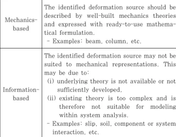
Mechanics- based

The identified deformation source should be described by well-built mechanics theories and expressed with ready-to-use mathema- tical formulation.

- Examples: beam, column, etc.

Information- based

The identified deformation source may not be suited to mechanical representations. This may be due to:

(i) underlying theory is not available or not sufficiently developed,

(ii) existing theory is too complex and is therefore not suitable for modeling within system analysis.

- Examples: slip, soil, component or system interaction, etc.

Table 1 Classification of components in hybrid modeling framework

The details will be illustrated in the following sections.

3.2 Classification of components

In the hybrid modeling formulation, it is important to establish how a mathematical model is comple- mented by informational methods or how both models are combined. This greatly influences implementation in current analysis tools, such as finite element analysis. In essence hybrid modeling adopts the concept of a component-based modeling approach. A component could be defined as not only a part, but also a group of parts, that comprise the system to be modeled. Components have their own constitutive relationships and their behaviors should critically affect the behavior of the system they comprise.

Therefore, identifying deformation sources is the initial step in the modeling process. Depending on the characteristics of each deformation source, components are classified to mechanics-based or information- based components.

After all components are classified as either mechanics-based or information-based, a mathe- matical model of the system is built first with the mechanics-based components. A mathematical model is based on the superposition of the contribution of the mechanics-based components, of which constitutive relationships are defined in mathematical formula-

tions. Though the mathematical model is expected to keep main stream or backbone trend of the system behavior, it inevitably involves a certain level of abstraction. It is modeling information-based comp- onents that can bridge the gap between the abstrac- tion and the reality. Details are given strictly within structural analysis.

3.3 Autoprogressive algorithm

In hybrid modeling framework, the adoption of autoprogressive algorithm(Ghaboussi et al., 1998) enables the constitutive models in component or material level to be updated by using the response in a system level. The autoprogressive algorithm extracts approximate constitutive information of components from the measured response of a system. The training data built with the difference between a mathematical model and the measured response in hybrid modeling formulation is obtained.

In the autoprogressive algorithm, global deforma- tion is measured with corresponding known external loads. A numerical simulation is developed with unknown constitutive models like a stress-strain material model. The unknown constitutive relation- ship is modeled with neural networks. This neural network is pre-trained with available a priori know- ledge, which may not accurately represent the material behavior. In the autoprogressive cycles, two forward analyses of inputting a discrete load and displacement yield approximate(but presumably improved) stress- strain training cases. The neural network material model is trained and updated with newly collected stress-strain training pairs. These forward analyses and training are iterated at each load step until the structural level response is predicted accurately enough. This process, called autoprogressive iteration, is repeated through the full range of applied loads.

Care should be exercised in choosing the number of autoprogressive training cycles. Covering the full range of loads is referred to as a load pass. To complete training of neural network material models with satisfaction, several load passes may be required.

A: Force Controlled Analysis

B: Displacement Controlled Analysis

σ ^Training ε

Database

< F, d >

Global Measurement (stress-strain resultant domain)

< σ, ε >

Stress strain constitutive model A: Force

Controlled Analysis

B: Displacement Controlled Analysis

σ ^Training ε

Database A: Force

Controlled Analysis

B: Displacement Controlled Analysis σ

σ ^Training εε Database

< F, d >

Global Measurement (stress-strain resultant domain)

< F, d >

Global Measurement (stress-strain resultant domain)

< σ, ε >

Stress strain constitutive model

< σ, ε >

Stress strain constitutive model

Fig. 3 Autoprogressive algorithm

RO

RO RO RO

RO RO

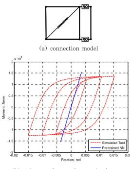
(a) connection model

-0.02-2 -0.015 -0.01 -0.005 0 0.005 0.01 0.015 0.02 -1.5

-1 -0.5 0 0.5 1 1.5

2x 10⁸

Rotation, rad

Moment, Nmm

Simulated Test Pre-trained NN

(b) reference data and pretrained curve Fig. 4 Hypothetical connection

control forward analysis(FCA), displacement control forward analysis(DCA), autoprogressive iteration, and several load passes -are also called self-learning simulation. The data flow from global measurements in the force-displacement domain to neural network material models in the stress-strain domain is illus- trated in Fig. 3.

4. Application examples

The challenge of modeling the behavior of beam-to- column connections in steel frames lies in the inelastic responses of individual components and their interac- tions. Some deformation components such as angles and flange-plates can be modeled with acceptable satisfaction by using only mechanical properties, while others such as slip and ovalization are more suitable for informational modeling.

4.1 Example 1: Mathematically generated data

To demonstrate that the hybrid modeling is effectively characterized in complex hysteretic behavior and to describe the model updating process, a hypothetical example of a beam-to-column connection is first considered instead of a real experimental test.

The hypothetical example is simulated with a mathematically based model. As seen in Fig. 4(a), a component-based model consists of two nonlinear

springs for connecting elements, a linear spring for the shear panel zone, and rigid bars. The nonlinear spring is formulated with a Ramberg-Osgood type function in the hypothetical model and this will be the target component behavior to be modeled by neural networks in a hybrid model. Fig. 4(b) shows the simulated moment-rotation curve of the whole connec- tion. This will be the reference data in hybrid modeling. Therefore, the self-learning simulation will extract the force-displacement relationship for the connecting component from moment-rotation reference data of the whole connection.

4.1.1 Hypothetical reference data

In order to create the hypothetical structural response data, an analytical Ramberg-Osgood model was used to represent the 1-D force-displacement behavior of the connecting members:

n n

f d K

d

f K

0 0 0

1 ⎟ ⎟

⎠

⎞

⎜ ⎜

⎝

⎛

⎟⎟ ⎠

⎜⎜ ⎞

⎝ + ⎛

=

where  is the initial stiffness,

^

^

For computational considerations, the tangent stiffness

Pass Number of converged load steps

Number of existing training cases

1 134 50

2 66 134

3 114 134

4 57 134

5 205 134

6 59 205

7 59 205

8 179 205

9 99 205

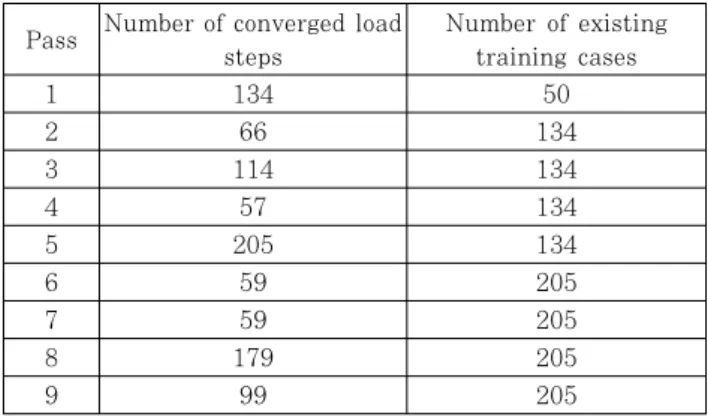
Table 2 Collection of training cases in model updating

Taking the derivative of the above equation with respect to the displacement, the following equation is obtained:

n n t

f d K

K K

1

0 0 0

1

+

⎟ ⎟

⎠

⎞

⎜ ⎜

⎝

⎛

⎟⎟ ⎠

⎜⎜ ⎞

⎝ + ⎛

=

where  is the tangent stiffness modulus expressed explicitly in terms of displacement and the three Ramberg-Osgood parameters. The following parameter values were selected: 



^



✕10⁵N;

^{ }

4.1.2 Neural network component model

For this example, a neural network is supposed to represent a smooth but not-pinched inelastic hysteretic behavior for the connecting components. The input layer has 5 nodes including the current axial displace- ment, the previous axial displacement and force, and two hysteretic parameters, and the output layer has 1 node of the current axial force. Two hidden layers are used and 15 nodes are assigned to each hidden layer.

The compact description of the architecture of a neural network component model is as follows:





 ^







∆

         

4.1.3 Elastic pre-training

Before starting the self-learning simulation, the neural network component model should be initialized.

The neural network is pre-trained on a data set generated from a linear elastic constitutive model, rather than assigning random initial connection weights.

In this example, 160 pairs of pre-training cases are generated randomly by using linear stiffness (665,072N/mm), with axial displacement lying in the range of(-0.6 : 0.6mm). The pre-training data set consists of 4 consecutive subsets, constructing a four-cycled response data. Each subset contains 40 training cases and is bounded by the gradually

increased range. The pretrained curve using the overall pre-training data set is illustrated in Fig.

4(b). The connection weights are initialized randomly at the beginning and then updated during the training. The inelastic behavior will then be captured through the next steps of the self-learning simulation.

4.1.4 Model updating in hybird modeling Table 2 presents the process of data collecting in updating the hybrid model. The second column shows the number of load steps, where both solutions loops of FCA and DCA converge. The third column shows the number of training cases in the training database, which is taken over from one of the previous passes.

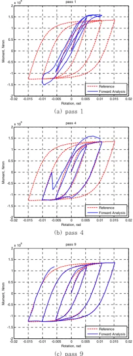
Before pass 1 starts, the training database contains 50 pre-training cases. Throughout the pass, new training cases are added to the training database at each converged load step. Before pass 2 begins, the training database contains 134 newly-collected training cases through pass 1. Until pass 5, the number of converged load steps is less than that of pass 1. This may imply that the solution loops cannot converge with the newly updated neural network model and therefore the newly-collected training cases may not be good candidates. Although 205 training cases are collected after pass 5, the training database keeps being updated by being replaced with the newly- collected training cases until the pass 9. Fig. 5 shows the evolution of moment-rotation curves by using the updated hybrid model at each pass.

The collected information is stored in the neural network for the informational components. Finally,

-0.02 -0.015 -0.01 -0.005 0 0.005 0.01 0.015 0.02 -2

-1.5 -1 -0.5 0 0.5 1 1.5

2x 10⁸

Rotation, rad

Moment, Nmm

pass 1

Reference Forward Analysis

(a) pass 1

-0.02 -0.015 -0.01 -0.005 0 0.005 0.01 0.015 0.02 -2

-1.5 -1 -0.5 0 0.5 1 1.5

2x 10⁸

Rotation, rad

Moment, Nmm

pass 4

Reference Forward Analysis

(b) pass 4

-0.02 -0.015 -0.01 -0.005 0 0.005 0.01 0.015 0.02 -2

-1.5 -1 -0.5 0 0.5 1 1.5

2x 10⁸

Rotation, rad

Moment, Nmm

pass 9

Reference Forward Analysis

(c) pass 9

Fig. 5 Evolution in model updating

a hybrid model is ready to predict the complex behavior of beam-to-column connections.

4.2 Example 2: Actually measured test data of a top-and-seat angle connection

4.2.1 Experimental tests

Full scale experimental tests of bolted connections were carried out by Bernuzzi et al.(1996). A top- and-seat angle connection labeled as TSC/D is chosen

for the purpose of hybrid modeling and its validation.

The specimen consists of a long beam stub of an IPE 300 section and a rigid counter-beam, which is regarded as a column but the deformation of column flanges and panel zone is disregarded. The loads are applied to the free end of the specimen by means of a device that transfers horizontal forces only. The loading history refers the recommendations approved by the European Convention for Constructional Steelwork(ECCS, 1986) but it allows only one cycle at the same level of displacement ratio. All bolts were grade 8.8 bolts fully preloaded according to the Italian code 4. Tension coupon tests for angles were conducted to determine the yield(313N/mm²) and ultimate (459N/mm²) strength.

4.2.2 Mathematical model

A mathematical model is built by using only material and geometric properties. The angles are idealized to a one-dimensional and tri-linear spring.

The panel zone is idealized as a linear spring with greater stiffness, as the deformability may be negligible.

The component describing the contact between the angles and the column flange is idealized to a one-dimensional linear spring with stiffness, which is approximately 15 times greater than the initial stiffness of the angle component in order to achieve negligible column deformation. The details of mathe- matical model could be refered to Kim et al.(2010).

4.2.3 Hybrid model

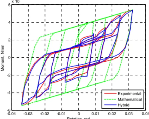
In a hybrid model as seen in Fig. 6, informational components illustrated with NN boxes are combined to the mathematical model composing of springs and rigid bars. The hybrid model is trained and updated by using actually measured test data. The moment- rotation curves of the experimental test, the mathe- matical model and the hybrid model are compared in Fig. 7. Although the curves from the experimental test and the mathematical model displays reasonable agreement in terms of initial and unloading stiffness, the hysteretic loops of the mathematical model do not include the pinching effects.

NN

NN NN

NN NN

NN

Fig. 6 Hybrid model of an angle connection

-0.04 -0.03 -0.02 -0.01 0 0.01 0.02 0.03 0.04

-6 -4 -2 0 2 4 6x 10⁷

Rotation, rad

Moment, Nmm

Experimental Mathematical Hybrid

Fig. 7 Comparison of moment-rotation curves of the angle connection

On the other hand, it is observed that the results of the hybrid model satisfactorily match the experi- mental results. In particular, the overall behaviors of both cases are characterized by the pinched shape, which are shown after the second cycle. Although the mathematical model cannot predict the pinching effects, the hybrid model combined with the information- based component is capable of representing those.

However, the curve of the hybrid model is not very smooth at the points corresponding to radians -0.02 and -0.03, when the slip reaches the face of the bolt hole and the overall responses are stiffened. This may be remedied through obtaining more reliable training data for the information-based component.

5. Conclusion

A information-based hybrid modeling framework, in this study, is developed for the purpose of realistic simulation. The basic premise of the developed metho- dology is that not all features of system response are amenable to mathematical modeling; hence conside- ring informational alternatives. In the hybrid mode-

ling framework, a mathematical model is updated by being complemented with the neural network compo- nent models, which are trained with the information that the mathematical model leaves out. The fitted self-learning simulation makes this possible.

The potential of hybrid modeling is demonstrated in two application examples. One mathematically gene- rated hypothetical example and the other actual experimental test of a top-and-seat angle connection are used for reference data in self-learning simula- tions. As a result, the mathematical model exhibits only smooth hysteretic behavior without pinching effects, while the hybrid model is capable of represen- ting all important aspects including pinching effects and mild degradation in stiffness.

참 고 문 헌

Bernuzzi, C., Zandonini, R., Zanon, P. (1996) Experimental Analysis and Modelling of Semi-Rigid Steel Joints under Cyclic Reversal Loading, Journal of Constructional Steel Research, 38(2), pp.95～

123.

Ghaboussi, J., Garrett, J.H., Wu, X. (1990) Material Modeling with Neural Networks, Procee- dings of the International Conference on Numerical Methods in Engineering: Theory and Applications, pp.701～717.

Ghaboussi J., Garrett J.H., Wu X. (1991) Knowledge-based Modeling of Material Behavior with Neural Networks, Journal of Engineering Mechanics, 117(1), pp.132～53.

Ghaboussi J., Zhang M., Wu X., Pecknold D.

(1997) Nested Adaptive Neural Network: A New Architecture, Proceedings of International confe- rence on Artificial Neural Networks in Engin- eering, ANNIE97, St. Louis, MO.

Ghaboussi J., Sidarta D.E. (1998) New Nested Adaptive Neural Networks (NANN) for Constitutive Modeling, Computers and Geotechnics, 22(1), pp.29

～52.

Ghaboussi, J., Pecknold, D.A., Zhang, M., &

Haj-Ali, R.M. (1998) Autoprogressive Training of Neural Network Constitutive Models, International Journal for Numerical Methods in Engineering,

42(1), pp.105～126.

Hashash, Y.M.A., Marulanda, C., Ghaboussi, J., Jung, S. (2003) Systematic Update of a Deep Excavation Model Using Field Performance Data, Computers and Geotechnics, 30(6), pp.477～488.

Hashash, Y.M.A., Marulanda, C., Ghaboussi, J., Jung, S. (2006) Novel Approach to Integration of Numerical Modeling and Field Observations for Deep Excavations, Journal of Geotechnical and Geoenvironmental Engineering, 132(8), pp.1019～

1031.

Kim, J.H., Ghaboussi, J., Elnashai, A.S. (2010) Mechanical and Informational Modeling of Steel

Beam-to-Column Connections, Engineering Stru- ctures, 32(2), pp.449～458.

Shin, H.S., Pande, G.N. (2000) On self-learning Finite Element Codes Based on Monitored Response of Structures, Computers and Geotechnics, 27(3), pp.161～178.

논문접수일 2012년 7월 5일

논문심사일 2012년 7월 9일

게재확정일 2012년 7월 23일