Print ISSN: 2288-4637 / Online ISSN 2288-4645 doi:10.13106/jafeb.2018.vol5.no3.19
Jensen’s Alpha Estimation Models in Capital Asset Pricing Model
Le Tan Phuoc
1Received: June 21, 2018 Revised: July 3, 2018 Accepted: July 30, 2018
Abstract
This research examined the alternatives of Jensen’s alpha (α) estimation models in the Capital Asset Pricing Model, discussed by Treynor (1961), Sharpe (1964), and Lintner (1965), using the robust maximum likelihood type m-estimator (MM estimator) and Bayes estimator with conjugate prior. According to finance literature and practices, alpha has often been estimated using ordinary least square (OLS) regression method and monthly return data set. A sample of 50 securities is randomly selected from the list of the S&P 500 index. Their daily and monthly returns were collected over a period of the last five years. This research showed that the robust MM estimator performed well better than the OLS and Bayes estimators in terms of efficiency. The Bayes estimator did not perform better than the OLS estimator as expected.
Interestingly, we also found that daily return data set would give more accurate alpha estimation than monthly return data set in all three MM, OLS, and Bayes estimators. We also proposed an alternative market efficiency test with the hypothesis testing Ho: α = 0 and was able to prove the S&P 500 index is efficient, but not perfect. More important, those findings above are checked with and validated by Jackknife resampling results.
Keywords: Jensen’s Alpha, Market Efficiency, Capital Asset Pricing Model, Bayes Estimator, Jackknife Resampling Methodology.
JEL Classification Code: C11, C15, G14.
1. Introduction 1
The Jensen’s alpha (α) introduced by Jensen (1967, 1969). This metric is used to measure the risk-adjusted return of a security or a portfolio of securities in line with the expected market return from Capital Asset Pricing Model (CAPM) discussed by Treynor (1961), Sharpe (1964), and Lintner (1965). The higher the alpha, the better performance of security or a portfolio of securities since it has earned more than expected return in Capital Asset Pricing Model.
The existence of this alpha (α) or abnormal return of a securities or portfolio of securities in worldwide financial markets has been documented by Jensen (1967 & 1969) himself, Kothari and Warner (1997a, 1997b), Liang (2008), Gerber and Hensz (2009), and many other researchers in the literature. Therefore, alpha becomes one of the key risk metrics used in the modern portfolio theory as stated in Association for Investment Management and Research
1 First Author and Corresponding Author. Lecturer, Becamex Business School, Eastern International University, Vietnam [Postal Address: Nam Ky Khoi Nghia Street, Hoa Phu Ward, Thu Dau Mot City, Binh Duong Province, Vietnam]
E-mail: Phuoc.le@eiu.edu.vn
(AIMR) performance presentation standards handbook (1996) even though it has deficiency as discussed in Black, Jensen, and Scholes (1972).
Some investors spend great time to locate a security or a portfolio of securities that has a positive alpha (α), especially in non-efficient markets. This strategy becomes one of the investment strategies for active investors. Hence, alpha estimation methods are critical to those investors. In practices as well as in finance literature, the alpha (α) has often been estimated with ordinary least square (OLS) estimator and monthly data set. However, the returns of security are known to be not normally distributed, especially with small sample size data set as Fama (1965), McDonald and Nelson (1989), and Martin and Simin (1999) pointed out in their research. This raised some concerns about the validity of alpha (α) estimate and investment decision making process with the ordinary least square estimator.
In light of recent research of Le, Kim, and Su (2018), we wanted to study the efficiency of alpha (α) estimation with alternative methods, the robust maximum likelihood type m- estimator (MM estimator) developed by Huber (1964, 1973) and Yohai (1985, 1987) and the Bayes estimator with conjugate prior, comparing with OLS estimator in this paper.
We also wanted to find out whether the monthly or daily data with the same estimator will yield better alpha
estimation. Based on the alpha (α) we wanted to estimate, we also proposed a different method to test the market efficiency. This test is the alpha (α) based test with the hypothesis testing : α = 0. We expected that in an efficient market, the alpha (α) = 0 as Jensen (1967 & 1969) discussed in his work. To address our research objectives, we applied the MM and Bayes estimators and both daily and monthly data sets to estimate alpha (α), its standard deviation, and its confidence interval or p value for hypothesis testing : α = 0 in this paper. We then compared them with the OLS estimator’s results. To validate our findings, we then checked with the results from the Jackknife resampling method developed by Tukey (1962) and has been applied by Bowie and Bradfield (1998) and Le, Kim, and Su (2018) in their work.
To help our readers, we divided this paper into 5 sections.
Section 1 is the Introduction. Section 2 is the Literature Review. Section 3 is the Data and Empirical Results. In this section, we would examine the normality assumption of both daily and monthly data with Kolmogorov-Smirnov goodness- of-fit tests. Then the empirical alpha (α), standard deviation, confidence interval or p value are estimated and scrutinized with both daily and monthly return data and the MM, OLS, and Bayes estimators. At the end of this section, the Jackknife resampling method was used to check and validate the findings above. In Section 4, the final Conclusions of this research are presented. The Section 5 is for the References and Appendix.
2. Literature Review
Jensen (1967, 1969) proposed to add the y-intercept coefficient, namely alpha (α), to Capital Asset Pricing Model to explain the possibility of superior forecasting knowledge from investors picking the securities that earned more than the risk premium for their levels of risks in Capital Asset Pricing model. Therefore, this Capital Asset Pricing Model can be written as follows:
For the security i = 1, 2, ..., n, we have
( ) − = + ( ) − + ( ) (1) where,
t is the date (day, week, or month) of each pair of observations,
is the return on the security i,
is the risk free rate,
is the alpha of security i, the security’s expected excess return when the market excess return is zero ( equals zero in an efficient market),
is the return of the market index,
βi = cov[( ( ) − ), ( ( ) − )] ÷ , the security’s sensitivity to the market index,
is the random error term of the security i that has mean zero; it is the firm-specific surprise in the security return.
From the equation (1) above, we can regress [( ( )− )] against [( ( ) − )] to determine alpha (α).
However, regression methods with different estimators could yield different results. Practitioners and researchers have often applied ordinary least square regression (OLS), assuming that the data is normally distributed, to estimate alpha (α) due to two main reasons. The first reason is the availability of the software that has the OLS function such as the Excel. The other reason is that the OLS regression will produce the best linear unbiased estimators (BLUE).
However, the assumption of the data is normally distributed is not satisfied as Fama (1965), McDonald and Nelson (1989), and Martin and Simin (1999) have proved in their research. This means that the alpha (α) estimate from the OLS estimator is not reliable and efficient and therefore could undermine investment decisions of investors.
To address this non-normal data, one option is to transform the data with the log function in order to stabilize the variance. Jensen (1967 & 1969) had applied the log function to transform the data and then estimate the alpha (α). Other researchers favored to estimate alpha (α) with other estimators rather than using the transformation function. Hwang and Salmon (2001) proposed the quantile regression (QR) estimator to estimate alpha (α) and other key metrics due to the non-normal distribution data. Trzpiot (2013) proposed to use least trimmed square (LTS) estimator and quantile regression (QR) estimators to estimate alpha (α) and proved that the least trimmed square estimator produced smaller standard deviation than ordinary least square estimator, but the QR estimator performed poorer, bigger standard deviation, than the OLS estimator in term of efficiency. Musumeci in his draft (2016) suggested that different way to estimate alpha (α). That is to estimate other coefficient, namely beta (β), in the CAPM first then use this beta (β) estimate to find the alpha (α). To estimate this beta (β), Musumeci considered all the observations except the ones that lead the market risk premium is unusually different from the mean because the abnormal performances are likely to distort beta (β) estimate and then alpha (α) estimate as well.
3. Data Description and Empirical Results
A sample of 50 individual securities is randomly selected from member securities of the S&P 500 index. These securities daily and monthly returns were collected over a period of the last five years as Alexander and Chervany (1980), Theobald (1981), and Levy and Schwartz (1997) suggested in their research. The daily and monthly returns on Treasury Bills were also collected and used as risk-free rate in this same period as Ross, Westerfield, and Jordan (2006) and Bodie, Kane, and Marcus (2008), Le, Kim, and Su (2018), and many other researchers have suggested in their books and work. Then, both daily and monthly returns were analyzed with the robust MM, OLS, and Bayes estimators. The outcomes from the robust MM, OLS and Bayesian linear regressions were compared in terms of their efficiency between monthly and daily return data with the same estimator and between estimators with the same data.
The results are presented in the Section 3.1 – Section 3.5 below.
3.1. The Kolmogorov-Smirnov Goodness-of-Fit Tests
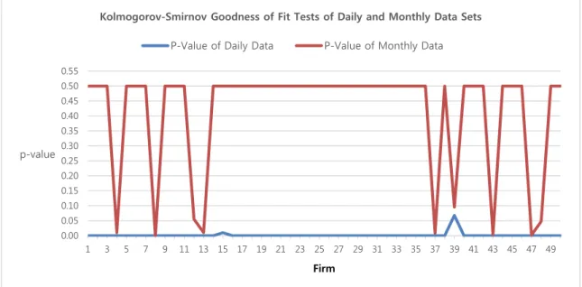
The Kolmogorov-Smirnov Goodness-of-Fit Tests of daily data and monthly data with the hypothesis testing H0: the data is normally distributed are presented below. With the significant level is 5%, the Figure 1 below shows that for daily data, there are 49 out of 50 firms’ returns are not normally distributed since their p values are less than
significant level 5%. This finding is agreed with what Fama (1965) pointed out. In contrast, for the monthly data there are only 7 out of 50 firms’ returns are not normally distributed since their p-values are less than 5%. This result from the monthly data is not surprised since monthly returns are the average of daily returns and therefore they are more stable than daily returns.
3.2. The Daily versus Monthly Alpha Estimate and Standard Deviation with OLS, MM, and Bayes Estimators.
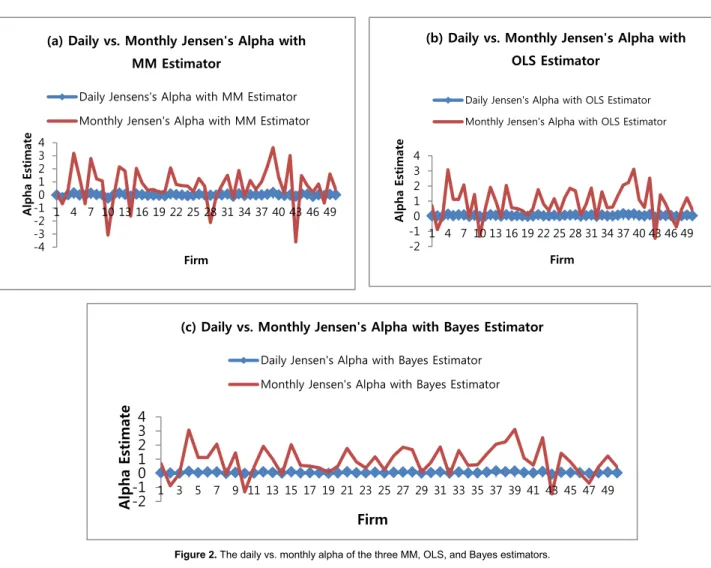
From the Figure 2 below, we can see very clearly that the fluctuation of alphas between firms with the MM, OLS, and Bayes estimators and monthly data are much greater than the daily data. A very interesting point we can see that for daily data, all the alphas with the MM, OLS and Bayes estimator are closed to and distributed around zero. In fact, the Figure 2a shows there are 25 out of 50 (50%) firms’
alpha are greater than zero with the MM estimator for daily data. The Figure 2b and the Figure 2c show that there are 45 out of 50 (90%) firms’ alphas are greater than zero with the OLS and Bayes estimators for daily data. For the monthly data, the Figure 2a shows that there are 39 out of 50 (78%) firms’ alpha are greater than zero with the MM estimator while there are 41 out of 50 (82%) firms’ alpha are greater than zero with OLS and Bayes estimators from the Figure 2b and Figure 2c. These findings are reinforced many claims in the literature that the Jensen’s alpha is really existed.
Figure 1. The Kolmogorov-Smirnov goodness-of-fit tests of daily and monthly data.
0.00 0.05 0.10 0.15 0.20 0.25 0.30 0.35 0.40 0.45 0.50 0.55
1 3 5 7 9 11 13 15 17 19 21 23 25 27 29 31 33 35 37 39 41 43 45 47 49 p-value
Firm
Kolmogorov-Smirnov Goodness of Fit Tests of Daily and Monthly Data Sets P-Value of Daily Data P-Value of Monthly Data
Figure 2. The daily vs. monthly alpha of the three MM, OLS, and Bayes estimators.
-2 -101 2 3 4
1 4 7 10 13 16 19 22 25 28 31 34 37 40 43 46 49
Alpha Estimate
Firm
(b) Daily vs. Monthly Jensen's Alpha with OLS Estimator
Daily Jensen's Alpha with OLS Estimator Monthly Jensen's Alpha with OLS Estimator
-4-3 -2-101234
1 4 7 10 13 16 19 22 25 28 31 34 37 40 43 46 49
Alpha Estimate
Firm
(a) Daily vs. Monthly Jensen's Alpha with MM Estimator
Daily Jensens's Alpha with MM Estimator Monthly Jensen's Alpha with MM Estimator
-2-101234
1 3 5 7 9 11 13 15 17 19 21 23 25 27 29 31 33 35 37 39 41 43 45 47 49
Alpha Estimate
Firm
(c) Daily vs. Monthly Jensen's Alpha with Bayes Estimator
Daily Jensen's Alpha with Bayes Estimator Monthly Jensen's Alpha with Bayes Estimator
0 1 2 3
1 4 7 10 13 16 19 22 25 28 31 34 37 40 43 46 49
Sta. Deviation Estimate
Firm
(b) Daily vs. Monthly Jensen's Alpha Sta. Deviation with OLS Estimator
Daily Jensen's Alpha Sta. Deviation with OLS Estimator
Monthly Jensen's Alpha Sta. Deviation with OLS Estimator
0 1 2 3 4
1 4 7 1013161922252831343740434649
Sta. Deviation Estimate
Firm
(a) Daily vs. Monthly Jensen's Alpha Sta. Deviation with MM Estimator
Daily Jensen's Alpha Sta. Deviation with MM Estimator
Monthly Jensen's Alpha Sta. Deviation with MM Estimator
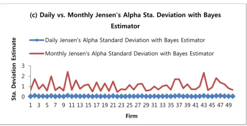
Figure 3. The daily vs. monthly alpha standard deviation of the three MM, OLS, and Bayes estimators.
More interesting findings can be observed from the Figures 3. The first one is all (100%) the alpha standard deviations with the MM, OLS, and Bayes estimators and monthly data are much greater than the daily data. The second one is for daily data, all the alpha standard deviations with the MM, OLS and Bayes estimator are closed to and distributed around zero. These findings show that alpha estimation with daily data will be more efficient and stable for all three estimators in this study. Therefore, the daily data is recommended over the monthly data in alpha estimation and analysis processes. Hence, the rest of this paper will consider only daily data in alpha inferences.
3.3. Daily Alpha Estimate and Standard Deviation with the Three OLS, MM, and Bayes Estimators
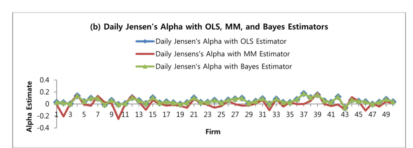
With the Figure 4, it is very interesting to see that the OLS and Bayes estimators produced almost identical alpha estimates and standard deviations as not expected. This sounds like a contradiction with many claims in the Bayesian school of thought that the Bayes estimator is often more efficient than the OLS estimator. With a close look at Figure 4a, we can find out that there are 43 out of 50 (86%) firms’ alpha standard deviations with MM estimator are smaller than with OLS and Bayes estimators. This means that the MM estimator is more efficient than the OLS and Bayes estimators and should be considered in alpha estimation.
0 1 2 3
1 3 5 7 9 11 13 15 17 19 21 23 25 27 29 31 33 35 37 39 41 43 45 47 49
Sta. Deviation Estimate
Firm
(c) Daily vs. Monthly Jensen's Alpha Sta. Deviation with Bayes Estimator
Daily Jensen's Alpha Standard Deviation with Bayes Estimator Monthly Jensen's Alpha Standard Deviation with Bayes Estimator
0 0.1 0.2
1 3 5 7 9 11 13 15 17 19 21 23 25 27 29 31 33 35 37 39 41 43 45 47 49
Sta. Deviation Estimate
Firm
(a) Daily Jensen's Alpha Sta. Deviation with OLS, MM, and Bayes Estimators
Daily Jensen's Alpha Sta. Deviation with OLS Estimator Daily Jensen's Alpha Sta. Deviation with MM Estimator Daily Jensen's Alpha Standard Deviation with Bayes Estimator
Figure 4. The comparisons of daily alpha and sta. deviation with MM, OLS, and Bayes estimators.
3.4. The Market Efficiency Test
The market efficiency test with hypothesis testing ( : α = 0 ) and alpha confidence interval from Bayes estimator. With the significant level is 5%, the Figure 5a shows that there are 44 out of 50 (88%) and 41 out of 50 (82%) firms’ p- values are greater than significant level 5% with the OLS and MM estimators respectively. This means that we do not have enough evidence to reject : α = 0 for the majority of
these 50 firms. The similar result can be obtained from the Figure 5b with the 95% confidence interval of alpha with Bayes estimator. There are 44 out of 50 (88%) firms’ alpha confidence intervals that contain zero. Hence, we cannot reject : α = 0. Therefore, we can conclude that there are strong evidences to claim that the S&P 500 index is efficient, but not perfect. This reinforces the arguments that the Jensen’s alpha is really existed and alpha estimation models selection is important to investors.
Figure 5. The efficient market hypothesis test with alpha.
-0.4 -0.2 0 0.2 0.4
1 3 5 7 9 11 13 15 17 19 21 23 25 27 29 31 33 35 37 39 41 43 45 47 49
Alpha Estimate
Firm
(b) Daily Jensen's Alpha with OLS, MM, and Bayes Estimators Daily Jensen's Alpha with OLS Estimator
Daily Jensens's Alpha with MM Estimator Daily Jensen's Alpha with Bayes Estimator
0.000.05 0.100.15 0.200.25 0.300.35 0.400.45 0.500.55 0.600.65 0.700.75 0.800.85 0.900.95 1.001.05
1 3 5 7 9 1113151719212325272931333537394143454749
p-vvalue
Firm
(a) The Daily P-Value of the Market Efficient Test with Hypothesis Testing Ho: Alpha = 0
Daily p-value with OLS estimator Daily p-value with MM estimator
-0.3 -0.2 -0.1 0 0.1 0.2 0.3 0.4
1 4 7 1013161922252831343740434649
Firm
(b) Daily 95% Confidence Interval of Alpha with Bayes Estimator
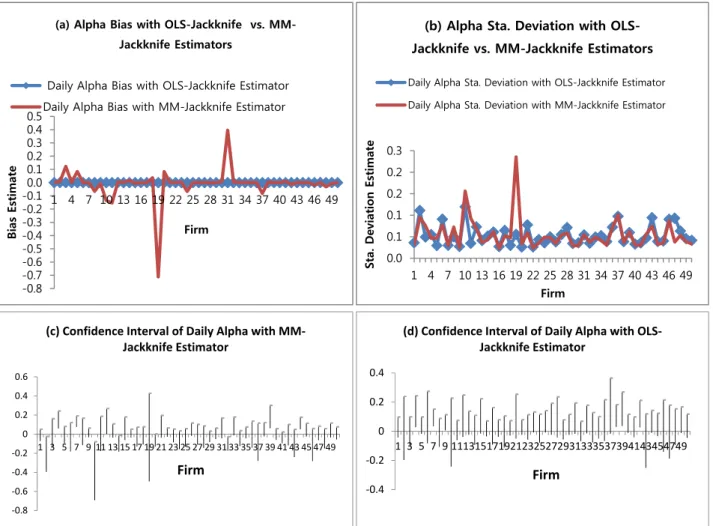
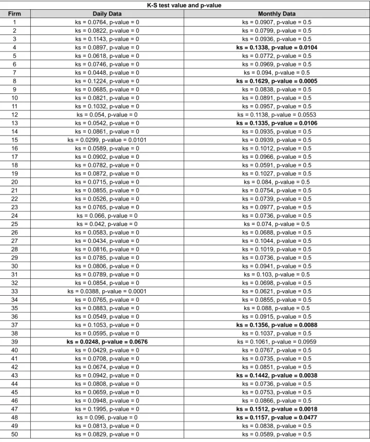
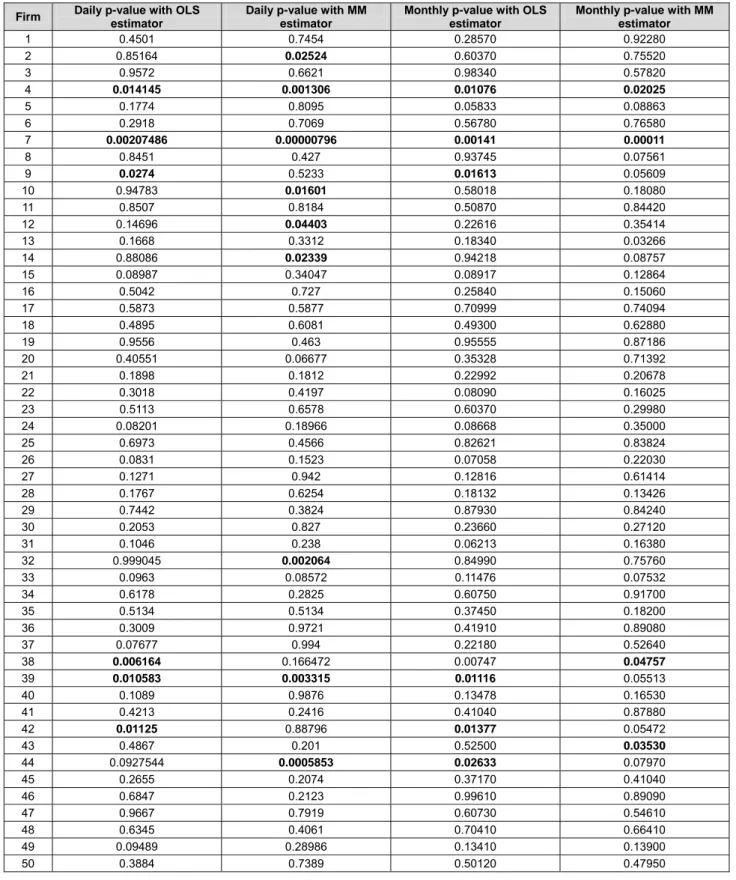
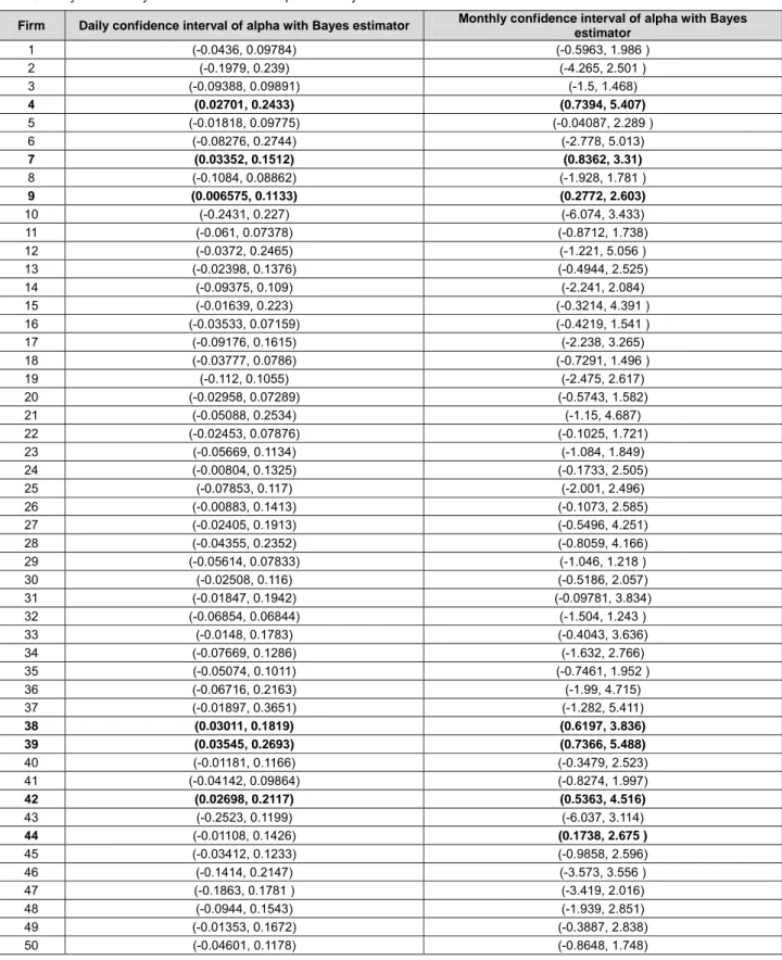
3.5. The Jackknife Resampling Methodology Results
In this section, we would like to validate those findings above by conducting a simulation with Jackknife resampling technique. With this method, the alpha coefficient of each firm is calculated for n possible times with one observation left out each time. If the Jackknife alpha estimates are closely the same, then the estimator is considered as efficient. The estimator is considered inefficient if the Jackknife alpha estimates exhibit high dispersion around the mean or there are many outliers. Therefore, we can assess the estimator's efficiency through two measurements: the bias and the standard error (standard deviation). The bias is the difference between the alpha estimate and the sample mean of Jackknife alpha estimates. The standard error
measures the dispersion from the alpha estimate. Therefore, it is considered a primary efficiency.
With the Figure 6a, we can see that 41 out of 50 (82%) firms’ alphas with OLS-Jackknife and MM-Jackknife estimators are much closed to each other. More important, the Figure 6b shows that 35 out of 50 (70%) firms’ alpha standard deviations with MM-Jackknife estimator are smaller than OLS-Jackknife estimator. This validated the conclusion above that the MM estimator is more efficient than the OLS estimator in alpha estimation. The Figure 6c and Figure 6d show that there are 42 out of 50 (82%) and 44 out of 50 (88%) firms’ alpha confidence intervals contained zero with MM-Jackknife and OLS-Jackknife estimators respectively. This again validated the conclusion above that there are strong evidences to claim the S&P 500 index is efficient, but not perfect.
Figure 6. The Jackknife resampling alpha bias, standard deviation, and the confidence intervals -0.8-0.7
-0.6-0.5 -0.4-0.3 -0.2-0.10.00.10.20.30.40.5
1 4 7 10 13 16 19 22 25 28 31 34 37 40 43 46 49
Bias Estimate
Firm
(a) Alpha Bias with OLS-Jackknife vs. MM- Jackknife Estimators
Daily Alpha Bias with OLS-Jackknife Estimator Daily Alpha Bias with MM-Jackknife Estimator
0.0 0.1 0.1 0.2 0.2 0.3
1 4 7 10 13 16 19 22 25 28 31 34 37 40 43 46 49
Sta. Deviation Estimate
Firm
(b) Alpha Sta. Deviation with OLS- Jackknife vs. MM-Jackknife Estimators
Daily Alpha Sta. Deviation with OLS-Jackknife Estimator Daily Alpha Sta. Deviation with MM-Jackknife Estimator
-0.4 -0.2 0 0.2 0.4
1 3 5 7 9 1113151719212325272931333537394143454749
Firm
(d) Confidence Interval of Daily Alpha with OLS- Jackknife Estimator
-0.8 -0.6 -0.4 -0.2 0 0.2 0.4 0.6
1 3 5 7 9 11 13 15 17 19 21 23 25 27 29 31 33 35 37 39 41 43 45 47 49
Firm
(c) Confidence Interval of Daily Alpha with MM- Jackknife Estimator
4. Conclusions
The both robust MM and Bayes estimators worked well in this study. However, the Bayes estimator yielded the almost identical results as the OLS estimators for both daily and monthly data. The robust MM-estimator outperformed both the OLS and Bayes estimators in estimation of Jensen’s alpha coefficients of securities listed in the S&P 500. Even the monthly return data are normally distributed, but all the firms’ alpha and alpha standard deviation estimates are much greater than daily return data for all three MM, OLS, and Bayes estimators. Therefore, the daily data is strongly recommended in Jensen’s estimation. The last conclusion is that there are strong evidences to support the claim that the S&P 500 index is efficient, but not perfect. This conclusion is agreed with other studies in the literature and general opinions from investors. Also, this conclusion gives a big hand to the arguments about the Jensen’s alpha existence.
Therefore, the Jensen’s alpha estimation models selection is important to investors.
References
Alexander, G. J., & Chervany, N. L. (1980). On the estimation and stability of beta. Journal of Financial and Quantitative Analysis, 15 (1), 123-137.
Association for Investment Management and Research (1996).
AIMR performance presentation standards handbook 1997.
2nd ed. Charlottesville: VA: The Association.
Black, F., Jensen, M. C., & Scholes, M. (1972). The capital asset pricing model: some empirical tests. Praeger Publishers Inc.
Retrieved from https://ssrn.com/abstract=908569
Bodie, Z., Kane, A., & Marcus, A. J. (2008). Investments. 7th ed.
New York: McGraw Hill/Irwin.
Bowie, D. C., & Bradfield, D. J. (1998). Robust estimation of beta coefficients: Evidence from a small stock market. Journal of Business Finance & Accounting, 25(3‐4), 439-454.
Fama, E. F. (1965). The behavior of stock market prices. Journal of Business, 38(1), 34-105.
Gerber, A. & Hensz, T. (2009). Jensen's alpha in the CAPM with heterogeneous beliefs. (National Centre of Competence in Research Financial Valuation and Risk Management No.
317). Retrieved from http://www.nccr-finrisk.uzh.ch/media /pdf/wp/WP317_A1.pdf.
Huber, P. J. (1964). Robust estimation of a location parameter.
Annals of Mathematical Statistics, 35, 73-101.
Huber, P. J. (1973). Robust regression: asymptotics, conjectures and Monte Carlo. Annals of Statistics, 1, 799-821.
Hwang, S., & Salmon, M. (2001). An analysis of performance measures using copulae. Retrieved from https://www.semanticscholar.org/paper/An-Analysis-of-
Performance-Measures-using-Copulae-Hwang-
Salmon/987908b45dd397c16256cb3641c73f6e4f732d7e Jensen, M. C. (1967). The performance of mutual funds in the
period 1945-1964. Journal of Finance, 23(2), 389-416.
Jensen, M. C (1969). Risk, the pricing of capital assets, and the evaluation of investment portfolios. The Journal of Business, 42(2), 167-247.
Kothari, S. P., & Warner, J. B. (1997a). Measuring long-horizon security price performance. Journal of Financial Economics, 43(3), 301-339.
Kothari, S.P., & Warner, J. B. (1997b). Measuring mutual fund
performance. Retrieved from https://ssrn.com/abstract=11176
Le, P. T., Kim, K. S., & Su, Y. (2018). Reexamination of estimating beta coefficient as a risk measure in CAPM. The Journal of Asian Finance, Economics, and Business, 5(1), 11-16.
Levy, H. & Schwarz, G. (1997). Correlation and the time interval over which variables are measured. Journal of Econometrics 76, 341-350.
Liang, P. (2008). Empirical study on the performance of initial public offerings in China. Journal of Service Science and Management, 1(2), 135-142.
Lintner, J. (1965). The valuation of risk assets and the selection of risky investments in stock portfolios and capital budgets.
Review of Economics and Statistics, 47, 13-37.
Martin, R. D. & Simin, T. (1999). Estimates of small-stock betas are often very distorted by outliers. Technical Report No. 351.
Department of Statistics – University of Washington.
McDonald, J. B., & Nelson, R. D. (1989). Alternative beta estimation for the market model using partially adaptive techniques.
Communications in Statistics, 18(11), 4039- 4058.
Musumeci, J. (2016). Jensen’s alpha - a problem and a solution.
Retrieved from http://www.efmaefm.org/0EFMAMEETINGS/
EFMA%20ANNUAL%20MEETINGS/2017- Athens/papers/EFMA2017_0495_fullpaper.pdf.
Ross, A. S., Westerfield, W. R., & Jordan, D. B. (2006).
Fundamentals of corporate finance. 7th ed. Boston:
McGraw-Hill.
Sharpe, W. F. (1964). Capital asset prices: a theory of market equilibrium under conditions of risk. Journal of Finance, 19(3), 425-442.
Theobald, M. (1981). Beta stationary and estimation period: some analytical results. Journal of Financial and Quantitative Analysis, 15 (5), 747-757.
Treynor, J. (1961). Towards a theory of the market value of risky assets. Unpublished manuscript.
Trzpiot, G. (2013). Selected robust methods for CAPM estimation.
Folia Oeconomica Stetinensia. 58-71.
Tukey, J. W. (1962). The future of data analysis. Annals of Mathematical Statistics 33:1- 67.
Yohai, J. V. (1985). High breakdown point and high efficiency robust estimates for regression. Technical Report, 66, 1-47.
Yohai, J. V. (1987). High breakdown point and high efficiency robust estimates for regression. The Annals of Statistics, 15(2), 642-656.
Appendix: Additional Tables
Table 1. The Kolmogorov-Smirnov goodness-of-fit tests of daily and monthly data.
K-S test value and p-value
Firm Daily Data Monthly Data
1 ks = 0.0764, p-value = 0 ks = 0.0907, p-value = 0.5 2 ks = 0.0822, p-value = 0 ks = 0.0799, p-value = 0.5 3 ks = 0.1143, p-value = 0 ks = 0.0936, p-value = 0.5 4 ks = 0.0897, p-value = 0 ks = 0.1338, p-value = 0.0104 5 ks = 0.0618, p-value = 0 ks = 0.0772, p-value = 0.5 6 ks = 0.0746, p-value = 0 ks = 0.0969, p-value = 0.5 7 ks = 0.0448, p-value = 0 ks = 0.094, p-value = 0.5 8 ks = 0.1224, p-value = 0 ks = 0.1629, p-value = 0.0005 9 ks = 0.0685, p-value = 0 ks = 0.0838, p-value = 0.5 10 ks = 0.0821, p-value = 0 ks = 0.0891, p-value = 0.5 11 ks = 0.1032, p-value = 0 ks = 0.0957, p-value = 0.5 12 ks = 0.054, p-value = 0 ks = 0.1138, p-value = 0.0553 13 ks = 0.0542, p-value = 0 ks = 0.1335, p-value = 0.0106 14 ks = 0.0861, p-value = 0 ks = 0.0935, p-value = 0.5 15 ks = 0.0299, p-value = 0.0101 ks = 0.0939, p-value = 0.5 16 ks = 0.0589, p-value = 0 ks = 0.1012, p-value = 0.5 17 ks = 0.0902, p-value = 0 ks = 0.0966, p-value = 0.5 18 ks = 0.0782, p-value = 0 ks = 0.0591, p-value = 0.5 19 ks = 0.0872, p-value = 0 ks = 0.1027, p-value = 0.5 20 ks = 0.0715, p-value = 0 ks = 0.084, p-value = 0.5 21 ks = 0.0855, p-value = 0 ks = 0.0754, p-value = 0.5 22 ks = 0.0526, p-value = 0 ks = 0.0739, p-value = 0.5 23 ks = 0.0765, p-value = 0 ks = 0.0977, p-value = 0.5 24 ks = 0.066, p-value = 0 ks = 0.0736, p-value = 0.5 25 ks = 0.042, p-value = 0 ks = 0.074, p-value = 0.5 26 ks = 0.0583, p-value = 0 ks = 0.0688, p-value = 0.5 27 ks = 0.0434, p-value = 0 ks = 0.1044, p-value = 0.5 28 ks = 0.0816, p-value = 0 ks = 0.1019, p-value = 0.5 29 ks = 0.0785, p-value = 0 ks = 0.0736, p-value = 0.5 30 ks = 0.0806, p-value = 0 ks = 0.0941, p-value = 0.5 31 ks = 0.0789, p-value = 0 ks = 0.103, p-value = 0.5 32 ks = 0.0854, p-value = 0 ks = 0.0698, p-value = 0.5 33 ks = 0.0388, p-value = 0.0001 ks = 0.0621, p-value = 0.5 34 ks = 0.0765, p-value = 0 ks = 0.0855, p-value = 0.5 35 ks = 0.0883, p-value = 0 ks = 0.088, p-value = 0.5 36 ks = 0.0549, p-value = 0 ks = 0.0915, p-value = 0.5 37 ks = 0.1053, p-value = 0 ks = 0.1356, p-value = 0.0088 38 ks = 0.0595, p-value = 0 ks = 0.1037, p-value = 0.5 39 ks = 0.0248, p-value = 0.0676 ks = 0.1061, p-value = 0.0959 40 ks = 0.0429, p-value = 0 ks = 0.0767, p-value = 0.5 41 ks = 0.0708, p-value = 0 ks = 0.0735, p-value = 0.5 42 ks = 0.0674, p-value = 0 ks = 0.0851, p-value = 0.5 43 ks = 0.0942, p-value = 0 ks = 0.1442, p-value = 0.0038 44 ks = 0.0808, p-value = 0 ks = 0.0736, p-value = 0.5 45 ks = 0.0659, p-value = 0 ks = 0.0753, p-value = 0.5 46 ks = 0.0948, p-value = 0 ks = 0.0866, p-value = 0.5 47 ks = 0.1995, p-value = 0 ks = 0.1512, p-value = 0.0018 48 ks = 0.096, p-value = 0 ks = 0.1157, p-value = 0.0477 49 ks = 0.0813, p-value = 0 ks = 0.0838, p-value = 0.5 50 ks = 0.0829, p-value = 0 ks = 0.0589, p-value = 0.5
Table 2. The daily and monthly p-value of the hypothesis testing Ho: alpha = 0.
Firm Daily p-value with OLS estimator
Daily p-value with MM estimator
Monthly p-value with OLS estimator
Monthly p-value with MM estimator
1 0.4501 0.7454 0.28570 0.92280
2 0.85164 0.02524 0.60370 0.75520
3 0.9572 0.6621 0.98340 0.57820
4 0.014145 0.001306 0.01076 0.02025
5 0.1774 0.8095 0.05833 0.08863
6 0.2918 0.7069 0.56780 0.76580
7 0.00207486 0.00000796 0.00141 0.00011
8 0.8451 0.427 0.93745 0.07561
9 0.0274 0.5233 0.01613 0.05609
10 0.94783 0.01601 0.58018 0.18080
11 0.8507 0.8184 0.50870 0.84420
12 0.14696 0.04403 0.22616 0.35414
13 0.1668 0.3312 0.18340 0.03266
14 0.88086 0.02339 0.94218 0.08757
15 0.08987 0.34047 0.08917 0.12864
16 0.5042 0.727 0.25840 0.15060
17 0.5873 0.5877 0.70999 0.74094
18 0.4895 0.6081 0.49300 0.62880
19 0.9556 0.463 0.95555 0.87186
20 0.40551 0.06677 0.35328 0.71392
21 0.1898 0.1812 0.22992 0.20678
22 0.3018 0.4197 0.08090 0.16025
23 0.5113 0.6578 0.60370 0.29980
24 0.08201 0.18966 0.08668 0.35000
25 0.6973 0.4566 0.82621 0.83824
26 0.0831 0.1523 0.07058 0.22030
27 0.1271 0.942 0.12816 0.61414
28 0.1767 0.6254 0.18132 0.13426
29 0.7442 0.3824 0.87930 0.84240
30 0.2053 0.827 0.23660 0.27120
31 0.1046 0.238 0.06213 0.16380
32 0.999045 0.002064 0.84990 0.75760
33 0.0963 0.08572 0.11476 0.07532
34 0.6178 0.2825 0.60750 0.91700
35 0.5134 0.5134 0.37450 0.18200
36 0.3009 0.9721 0.41910 0.89080
37 0.07677 0.994 0.22180 0.52640
38 0.006164 0.166472 0.00747 0.04757
39 0.010583 0.003315 0.01116 0.05513
40 0.1089 0.9876 0.13478 0.16530
41 0.4213 0.2416 0.41040 0.87880
42 0.01125 0.88796 0.01377 0.05472
43 0.4867 0.201 0.52500 0.03530
44 0.0927544 0.0005853 0.02633 0.07970
45 0.2655 0.2074 0.37170 0.41040
46 0.6847 0.2123 0.99610 0.89090
47 0.9667 0.7919 0.60730 0.54610
48 0.6345 0.4061 0.70410 0.66410
49 0.09489 0.28986 0.13410 0.13900
50 0.3884 0.7389 0.50120 0.47950
Table 3. Daily and monthly confidence interval of alpha with Bayes estimator.
Firm Daily confidence interval of alpha with Bayes estimator Monthly confidence interval of alpha with Bayes estimator
1 (-0.0436, 0.09784) (-0.5963, 1.986 )
2 (-0.1979, 0.239) (-4.265, 2.501 )
3 (-0.09388, 0.09891) (-1.5, 1.468)
4 (0.02701, 0.2433) (0.7394, 5.407)
5 (-0.01818, 0.09775) (-0.04087, 2.289 )
6 (-0.08276, 0.2744) (-2.778, 5.013)
7 (0.03352, 0.1512) (0.8362, 3.31)
8 (-0.1084, 0.08862) (-1.928, 1.781 )
9 (0.006575, 0.1133) (0.2772, 2.603)
10 (-0.2431, 0.227) (-6.074, 3.433)
11 (-0.061, 0.07378) (-0.8712, 1.738)
12 (-0.0372, 0.2465) (-1.221, 5.056 )
13 (-0.02398, 0.1376) (-0.4944, 2.525)
14 (-0.09375, 0.109) (-2.241, 2.084)
15 (-0.01639, 0.223) (-0.3214, 4.391 )
16 (-0.03533, 0.07159) (-0.4219, 1.541 )
17 (-0.09176, 0.1615) (-2.238, 3.265)
18 (-0.03777, 0.0786) (-0.7291, 1.496 )
19 (-0.112, 0.1055) (-2.475, 2.617)
20 (-0.02958, 0.07289) (-0.5743, 1.582)
21 (-0.05088, 0.2534) (-1.15, 4.687)
22 (-0.02453, 0.07876) (-0.1025, 1.721)
23 (-0.05669, 0.1134) (-1.084, 1.849)
24 (-0.00804, 0.1325) (-0.1733, 2.505)
25 (-0.07853, 0.117) (-2.001, 2.496)
26 (-0.00883, 0.1413) (-0.1073, 2.585)
27 (-0.02405, 0.1913) (-0.5496, 4.251)
28 (-0.04355, 0.2352) (-0.8059, 4.166)
29 (-0.05614, 0.07833) (-1.046, 1.218 )
30 (-0.02508, 0.116) (-0.5186, 2.057)
31 (-0.01847, 0.1942) (-0.09781, 3.834)
32 (-0.06854, 0.06844) (-1.504, 1.243 )
33 (-0.0148, 0.1783) (-0.4043, 3.636)
34 (-0.07669, 0.1286) (-1.632, 2.766)
35 (-0.05074, 0.1011) (-0.7461, 1.952 )
36 (-0.06716, 0.2163) (-1.99, 4.715)
37 (-0.01897, 0.3651) (-1.282, 5.411)
38 (0.03011, 0.1819) (0.6197, 3.836)
39 (0.03545, 0.2693) (0.7366, 5.488)
40 (-0.01181, 0.1166) (-0.3479, 2.523)
41 (-0.04142, 0.09864) (-0.8274, 1.997)
42 (0.02698, 0.2117) (0.5363, 4.516)
43 (-0.2523, 0.1199) (-6.037, 3.114)
44 (-0.01108, 0.1426) (0.1738, 2.675 )
45 (-0.03412, 0.1233) (-0.9858, 2.596)
46 (-0.1414, 0.2147) (-3.573, 3.556 )
47 (-0.1863, 0.1781 ) (-3.419, 2.016)
48 (-0.0944, 0.1543) (-1.939, 2.851)
49 (-0.01353, 0.1672) (-0.3887, 2.838)
50 (-0.04601, 0.1178) (-0.8648, 1.748)