Heuristics for Scheduling Wafer Lots at the Deposition Workstation in a Semiconductor Wafer Fab

Heuristics for Scheduling Wafer Lots at the Deposition Workstation in a Semiconductor Wafer Fab

Seong-Woo Choi

․Tae-Kyu Lim

․Yeong-Dae Kim

1

Department of Business Administration, Hoseo University, Cheonan-City, Choongnam 330-713, KOREA

2

Supply Planning Team, GS-Caltex Oil, GS Tower, Yoksam-dong, Kangnam-gu, Seoul 135-985, KOREA

3

Department of Industrial Engineering, Korea Advanced Institute of Science and Technology, Yusong-gu, Daejon 305-701, KOREA

반도체 웨이퍼 팹의 흡착공정에서 웨이퍼 로트들의 스케쥴링 알고리듬

최성우

․임태규

․김영대

1

호서대학교 경영학과 /

GS칼텍스 수급계획팀 /

한국과학기술원 산업공학과

This study focuses on the problem of scheduling wafer lots of several product families in the deposition workstation in a semiconductor wafer fabrication facility. There are multiple identical parallel machines in the deposition workstation, and two types of setups, record-dependent setup and family setup, may be required at the deposition machines. A record-dependent setup is needed to find optimal operational conditions for a wafer lot on a machine, and a family setup is needed between processings of different families. We suggest two-phase heuristic algorithms in which a priority-rule-based scheduling algorithm is used to generate an initial schedule in the first phase and the schedule is improved in the second phase. Results of computational tests on randomly generated test problems show that the suggested algorithms outperform a scheduling method used in a real manufacturing system in terms of the sum of weighted flowtimes of the wafer lots.

*

Keywords: Scheduling, Semiconductor Wafer Fabrication, Deposition, Heuristics

1. Introduction

In this paper, we consider a problem of scheduling wafer lots in the deposition workstation in a semiconductor wafer man- ufacturing system. A wafer lot is a group of wafers of the same type that are transported together and processed con- secutively in most workstations in a wafer fabrication facility (fab). Manufacturing process for semiconductor chips con- sists of four basic steps : wafer fabrication, wafer probe, as- sembly and test. (For detailed description of the semicon-

ductor manufacturing process, see Uzsoy et al., 1992.) Among these four, wafer fabrication is the most complex and time- consuming. Especially, the deposition process is a very im- portant (and time-consuming) process since it is closely re- lated to the yield and quality of products. Note that deposi- tion and photolithography workstations are considered as bottlenecks in general, although bottlenecks may vary ac- cording to the product-mix of the fab. It is important to oper- ate the bottleneck workstations effectively in order to im- prove the performance of the entire system. In this study, we focus on the deposition workstation.

This research was supported by the Academic Research fund of Hoseo University in 2009 (2009-0159).

†Corresponding author : Professor Kim Yeong-Dae, Department of Industrial Engineering, Korea Advanced Institute of Science and Technology, Yusong-gu, Daejon 305-701, KOREA Fax : +82-42-350-3110, E-mail : [email protected]

Received April 4, 2010; Revision Received May 13, 2010; Accepted May 18, 2010.

In the deposition workstation, there are multiple identical machines, that is, each wafer lot can be processed on one of the deposition machines, and each deposition machine can process only one wafer lot at a time. Wafer lots can be classi- fied into several product families in the deposition work- station according to their product specifications and chemical characteristics required for the deposition process. Since dep- osition is not the first operation of wafer fabrication, wafer lots arrive at this workstation dynamically. In other words, jobs (processing of wafer lots) may have different ready times in the scheduling problem for the deposition work- station. On the deposition machines, there exist two types of setups, family setup and record-dependent setup.

Family setup is required on each deposition machine be- fore a wafer lot of a family is processed, if it is processed af- ter a wafer lot of another family. In the deposition work- station, it is very important to control the thickness of each layer of the wafers, by which the quality and yield are af- fected significantly (although we do not deal with quality is- sues directly in this study). Therefore, optimal settings for the machines, such as injected vapor density, pressure and temperature, may be different for different families of wafer lots. Family setup is needed for setting an operational envi- ronment for a wafer family, and such a setup operation is executed by using data for optimal setting of a machine, which is obtained by another type of setup operations for the family and the machine.

On the other hand, record-dependent setup is required on a deposition machine according to the production record of the machine. In the fab considered in this study, it is called

“(production) history setup.” Since machine conditions change as time passes, an optimal setting for a pair of a machine and a wafer family is no longer optimal after a certain period of time even for the same machine and the same family. To ob- tain data for optimal setting of a machine and a family, en- gineers should process (dummy) wafers of the family at the machine and check the quality of the wafers completed. Such an operation is called the record-dependent setup or the his- tory setup. A record-dependent setup is required for the fam- ily on a machine, if a certain period of time has passed after a record-dependent setup was done on the machine. Note that the record-dependent setup is different from a (periodic) main- tenance executed on a machine. In general, maintenance op- erations are performed on a machine at (predetermined) time intervals for inside cleaning, parts inspection and replace- ments, and so on, regardless of wafer families that have been performed on the machine.

Also, note that a family setup is done for setting an opera- tional environment for wafer lots of a family on a machine by using data for optimal settings obtained by a (recent) re- cord-dependent setup. If there is no data for optimal setting for a wafer family and a machine when a family setup should be done on the machine, a record-dependent setup is needed for such data. In general, time required for a record-depend- ent setup is significantly long (longer than a family setup

time and the processing time of a wafer lot corresponding to the family) since engineers find the data for optimal setting by a series of test runs. Therefore, performance or productivity of the deposition workstation may be significantly affected by schedules of wafer lots, since frequencies of record-dependent setups on the machines are affected by the schedules. Both setups are separable, that is, even though a wafer lot is not ready for being processed on a machine, the setup operation for the wafer lot can be started on the machine if the machine is available.

At the time this research was conducted, main concerns of managers and engineers of the fab were the productivity of the fab and the work-in-process inventory (WIP). Since the deposition workstation is a subsystem of the whole semi- conductor manufacturing system, increasing throughput of a subsystem, or reducing flowtime of wafer lots may often help improve the performance of the whole system. In addition, in real systems, importance of different wafer lots may be dif- ferent according to their product types or processing urgen- cies. In this paper, we consider a problem of scheduling jobs, i.e., wafer lots, with distinct ready times and setup times on identical parallel machines with the objective of minimizing the sum of weighted flowtimes of the wafer lots, of which the weights are given according to their importance. Assum- ptions made in this problem are : (1) wafers of a wafer lot are processed together on a deposition machine; (2) no wafer lot can be preempted; (3) machines do not fail (there is no breakdown of the machines); and (4) ready times of wafer lots are known in advance.

There have been a number of studies on scheduling prob- lems in semiconductor wafer fabrication facilities, such as problems related to lot release control and lot scheduling at serial processing machines as well as batch processing machines. Lot release rules are developed in many studies in- cluding those of Wein (1998), Glassey and Resende (1988), Kim et al. (1998a, 1998b).

In these rules, information on the work load at a bottle- neck workstationis used for lot release. In most previous studies on lot scheduling problems with sequence-dependent setups in wafer fabs, dispatching rules have been used for se- quencing (Arzi and Raviv, 1998; Chern and Liu, 2003; Cigo- lini et al., 1999). Also, research on lot scheduling problems is focused on bottleneck workstations in most studies (Graves et al., 1983; Lou and Karger, 1989; Kim et al., 1998a, 1998b;

Lee et al., 1995; Min and Yih, 2003; Ko et al., 2004; Yoon and Lee, 2004; Lin et al., 2005). Batch scheduling problems have been dealt with in a few studies as well. For example, Glassey and Weng (1991) give a method for scheduling job of a single job family on a single batch processing machine, and Fowler et al. (1992), Robinson et al. (1995) and Fowler et al. (2000) deal with multi-product and multi-server cases.

Also, Kim et al. (1998b) suggest batch scheduling methods

to determine the number of lots to be produced simulta-

neously in a batch and the processing sequence of batches in

batch-processing workstations. For more details of research

on modeling and analysis of semiconductor wafer fabrica- tion, see survery papers of Uzsoy et al. (1992), Johri (1993), Duenyas et al. (1994) and Uzsoy et al. (1994).

As surveyed in Azizoglu and Kirca (1999), there are many studies on identical parallel machine scheduling problems with the objective of minimizing the sum of weighted flow- times (Eastman et al., 1964; Lawler and Moore, 1969; Bruno et al., 1974; Elmaghraby and Park, 1974; Barnes and Brennan, 1977; Lee and Uzsoy, 1992; Webster, 1993; Webster, 1994).

Also, there exist various algorithms developed for the prob- lem of scheduling jobs with family (not record-dependent) setups on identical parallel machines (Schutten and Leussink, 1996; Webster and Azizoglu, 2001; Azizoglu and Webster, 2003, Dunstall and Wirth, 2005a; Dunstall and Wirth, 2005b).

Note that this problem is NP-hard (Monma and Potts, 1989).

In addition, there are several research results on problems of scheduling jobs with distinct ready times on parallel ma- chines (Park and Kim, 1997; Dessouky, 1998;, Monch et al., 2005; Pfund et al., 2008). However, to the best of our kno- wledge, there is no study that deals with parallel machine scheduling problems with record-dependent setups. See Zhu and Wilhelm (2006) and Allahverdi et al. (2008) for com- plete reviews on research on scheduling problems with setup times.

In this paper, we present several heuristic algorithms for the problem of scheduling wafer lots with distinct ready times in a deposition workstation considering family setups as well as record-dependent setups for the objective of mini- mizing the sum of weighted flowtimes of the wafer lots. The suggested algorithms consist of two phases, those for initial schedule construction and schedule improvement. In the first phase, an initial schedule is obtained by scheduling methods modified from typical list scheduling algorithms, and the schedule obtained in phase 1 is improved in the second phase.

Note that algorithms with both phases can be used for static scheduling for a given scheduling horizon, while algorithms with only the first phase can be used not only for static scheduling but also for real-time scheduling or in a real-time dispatcher of a fab.

2. Heuristic Algorithms

In list scheduling algorithms, when a machine becomes available, an operation with the highest priority among oper- ations that can be processed on the machine at that moment is assigned to and processed on the machine. Also, when an operation becomes available and there are two or more ma- chines available for the operation at that moment, a machine with the highest priority is selected among those machines.

In this study, we modify the typical procedure of list schedul- ing algorithms to consider record-dependent setups in the first phase. In the second phase of the algorithms, schedules

are improved by left-shifts of jobs as well as changes of as- signments of wafer lots to machines and changes of se- quences of wafer lots on the machines. In addition to the above heuristic algorithms, we develop simulated annealing (SA) algorithms for the problem, which are to be used for evaluation of the performance of the heuristic algorithms.

Throughout the paper, we use the following notation.

i : index for wafer lots j : index for wafer families k : index for machines L : set of all wafer lots

A : set of wafer lots available currently (when the scheduling decision is to be made)

F : set of wafer families associated with wafer lots that can be processed (at the time when the sched- uling decision is to be made) after a record-depend- ent setup

K : set of the machines

k′ : index of a selected machine, i.e., the machine be- ing considered currently

[i] : index of the family corresponding to wafer lot i p

: processing time of wafer lot i (on the deposition

workstation)

R

: ready time of wafer lot i w

: weight of wafer lot i

s

: time required for a family setup, which is the same for all families



: time required for a record-dependent setup for family j

σ

: partial schedule of wafer lots that are already scheduled on machine k

C(σ

) : the time when all wafer lots in σ

are completed on machine k

e

: a parameter that is equal to 1 if a family setup is needed when wafer lot i is scheduled on machine k at time C(σ

), and 0 otherwise

E

: a parameter that is equal to 1 if a record-depend- ent setup is needed when a wafer lot of family j is scheduled on machine k at time C(σ

), and 0 oth- erwise

2.1 Phase 1: Schedule Construction

We present two approaches, a machine-based scheduling

approach and a lot-based scheduling approach. In both ap-

proaches, the basic concept of list scheduling algorithms is

employed. In the machine-based list scheduling algorithm

suggested in this study, when a machine becomes available,

priorities are computed for wafer lots that can be processed

on the machine at that time, and then a wafer lot with the

highest priority is scheduled on the machine. On the other

hand, in the lot-based list scheduling algorithm, when a ma-

chine becomes available, a wafer lot is selected with a certain

rule, and then the selected wafer lot is scheduled on a ma- chine that is selected with a machine priority rule.

The difference between the two approaches can be sum- marized as follows. In the lot-based approach, if there is at least one wafer lot available at the time when a machine be- comes available, we select a wafer lot to be scheduled and then we select a machine for the selected wafer lot. Therefore, a selected machine may not be the one that becomes avail- able earliest. However, in the machine-based approach, a ma- chine that becomes available earlier is scheduled earlier if there is a lot for the machine. Algorithms of both approaches include procedures for taking account of family setups as well as record-dependent setups.

(1) Machine-based list scheduling algorithm (MBLS) In this algorithm, the basic concept of the typical list scheduling method is employed. That is, if there is at least one available wafer lot (which can be processed without a re- cord-dependent setup) at the time when a machine becomes available, a wafer lot with the highest priority (selected with a lot priority rule) is selected and scheduled on the machine.

If the wafer family of the selected wafer lot is different from that of the wafer lot just processed on the machine, a family setup operation should be performed before the selected wa- fer lot is processed.

On the other hand, if there is no available wafer lot that can be processed without a record-dependent setup at the time when a machine becomes available, but there is at least one available wafer lot that can be processed after a re- cord-dependent setup, a wafer family with the highest prior- ity is selected among those associated with the available wa- fer lots by using a family priority rule. Then, a wafer lot with the highest priority is selected among those of the selected family, and scheduled on the machine after a record-depend- ent setup operation is done for the selected family. If there is no available wafer lot at all (with/without record-dependent setups) at the time when a machine becomes available, the scheduling decision is deferred until the time point when a wafer lot becomes ready or an other machine becomes available.

We present two lot priority rules and two family priority rules. The priority functions used for the rules are given below. Note that when a machine, say machine k', becomes available, the lot priority is computed for a pair of lot i and machine k' for i∈A, while the family priority is computed for a pair of family j and machine k' for j∈F. Here, |K| denotes the number of the machines.

a) Lot Priority Rules

LPR 1 : 

 

․ 



LPR 2 :   

 ≠ ^′





 

․ 



b) Family Priority Rules

FPR 1 :







FPR 2 :   

 ≠ ^′











Note that LPR1 is similar to the well-known weighted shortest processing time (WSPT) rule, in which a job (wafer lot) with the smallest value of p

/w

has the highest priority, but time required for a family setup is considered addition- ally in LPR1. In the priority function of LPR2,



 ≠^′



represents the number of machines, including the selected machine, on which a record-dependent setup is not needed for family [i] at the time when they become available. Therefore, if the priority function value of LPR2 is large for a lot, the lot has low priority on the machine since the wafer lot can be processed without record-dependent setups on other machines.

In both family priority rules, a higher priority is given to a family with a smaller sum of the weighted shortest process- ing times of available wafer lots of the family.

The procedure for this algorithm can be summarized as follows. Here, L denotes the set of wafer lots that have not been scheduled yet.

Procedure 1. (MBLS)

Step 0 : Let L be the set of all wafer lots.

Step 1 : If L = ∅, terminate. Otherwise, select a machine that becomes available earliest. Let t be the avail- able time of the selected machine k', i.e., t = min

∈K

C(σ

). Let A denote the set of wafer lots in L that can be processed without a record-dependent setup on the selected machine at t (those with ready times no later than t), and let F denote the set of wafer families associated with wafer lots in L that can be processed (after a record-dependent setup) on the selected machine at t.

Step 2 : If A = ∅, go to step 3. Otherwise, select a lot with the highest priority among those in A. Schedule the selected wafer lot on the selected machine (after a family setup, if needed), and update the available time of the machine as the completion time of the wafer lot. Delete the selected (and scheduled) wafer lot from L, and go to step 1.

Step 3 : If F≠∅, go to step 4. Otherwise, update the available time of the current machine as the min- imum ready time of wafer lots in L, i.e., min

L

R

, and go to step 1.

Step 4 : Select a wafer family with the highest priority among those in F. Schedule a record-dependent setup for (the family associated with) the se- lected wafer lot, and update the available time of the selected machine as the completion time of the record-dependent setup.

Step 5 : Compute priorities of wafer lots of the selected

family that become ready by the updated available

time of the selected machine, and then select a wafer lot with the highest priority. Schedule the selected wafer lot on the machine (after a family setup, if needed), and update the available time of the machine as the completion time of the wa- fer lot. Delete the selected (and scheduled) wafer lot from L, and go to step 1.

(2)Lot-based list scheduling algorithm (LBLS) In this algorithm, if a machine becomes available, a wafer lot is selected with a lot priority rule among those that are ready at the moment, to be denoted as t, and then the selected wafer lot is scheduled on a machine that is selected with a machine priority rule among all machines. Therefore, the se- lected machine may not be the one that becomes available earliest. That is, if the selected machine is not available at t, the selected lot is assigned to the machine but it will be sched- uled later (when the machine becomes available). When the selected lot is scheduled on the selected machine, a family setup or record-dependent setup operation should be sched- uled if needed.

In this study, we present three lot priority rules for LBLS and two machine priority rules, of which the priority func- tions are given below. Here, Q

denotes the number of the unscheduled wafer lots of family [i] that are available at the time when a machine becomes available. Note that the lot priority is computed for lot I, and the machine priority is computed for machine k (for a selected lot i' ).

a) Lot Priority Rules (for LBLS) LPR 3 : 



LPR 4 : 

 

․   





 

LPR 5 : 







b) Machine Priority Rules

MPR 1 : 

  





 

․ 

 

․ 

MPR 2 : 

  





 

․ 

 

․ 

   

 ≠ 



 Note that LPR3 is identical to the weighted shortest proc- essing time (WSPT) rule. In LPR4, record-dependent setup time is considered additionally, and if a wafer lot cannot be processed without a record-dependent setup on any machine, it is given a low priority. In LPR5, we give a higher priority to a wafer lot with more lots of the same family (as that of the wafer lot) available at the time when a machine becomes available. This is because it would be more likely that more lots (to be scheduled later on) can be processed without a re- cord-dependent or family setup, if a wafer lot with more lots of the same family is scheduled at the current time. In both machine priority rules, the highest priority is given to a ma- chine on which the selected wafer lot, lot i¢, can be com-

pleted earliest. Note that the term,



used in MPR2 is similar to the one used in LPR2. That is, for machine k,

 _{ ≠ }



represents the number of machines, including machine k, on which a record-dependent setup is not needed for family[i'] at the time when they become available.

Therefore, if the priority function value of a machine is larg- er, the machine is given a lower priority, since the selected lot can be processed without record-dependent setups on oth- er machines.

In the lot priority rules of MBLS (LPR1 and LPR2), prior- ities of the wafer lots are computed under the assumption that each of the wafer lot is scheduled on machine k', which is available at t. On the other hand, in the lot priority rules of LBLS (LPR3, LPR4, and LPR5), priorities of the wafer lots are computed without such an assumption. In these rules, the selected wafer lot is scheduled on the machine that is se- lected with a machine priority rule among all machines.

The procedure for this algorithm can be summarized as follows.

Procedure 2. (LBLS)

Step 0 : Let L be the set of all wafer lots.

Step 1 : If L=∅, terminate. Otherwise, let t be the avail- able time of a machine that becomes available earliest, i.e., t = min

C(σ

).

Step 2 : Let A be the set of wafer lots (in L) that become ready by time t. If A≠∅, go to step 3. Otherwise, update the available time of the machine as the minimum ready time of wafer lots in L, i.e., min

L

R

, and go to step 1.

Step 3 : Select a wafer lot with the highest priority among those in A. Select a machine with the highest pri- ority among all machines. Schedule the selected wafer lot on the selected machine with the highest priority among all machines (after a family setup or a record-dependent setup, if needed), and up- date the available time of the selected machine as the completion time of the wafer lot. Delete the se- lected (and scheduled) wafer lot from L, and go to step 1.

2.2 Phase 2: Schedule Improvement

A schedule obtained in the first phase is improved in the second phase with three improvement methods: left-shifts of the setup and processing operations, changes of the sequence on each machine (re-sequencing), and changes of the assign- ments of wafer lots to machines (re-assignment). Each meth- od is described in more detail in the following.

(1) Left-shift of the operations

Since the list scheduling method is used for scheduling in

the first phase, in a schedule obtained from the first phase, an

operation can be started only when a wafer lot and a machine

for the wafer lot become available. However, even though a wafer lot is not ready for being processed on a machine, the setup operation for the wafer lot can be started on the ma- chine if the machine is available. Therefore, we can improve the schedule by left-shift of such setup operations and oper- ations succeeding them. In this improvement method, if there is idle time that can be reduced by starting setup operations earlier on a machine, we shift operations affected by such setup operations to left (while considering the ready times of the wafer lots).

(2) Re-sequencing on each machine

In this improvement method, we consider the whole sched- ule as a set of m sub-schedules, one sub-schedule on each of m machines, and each sub-schedule is dealt with and im- proved individually using the basic concept of the algorithm of Nawaz et al. (1983), called NEH. That is, starting from the seed sequence, i.e., the sequence of the sub-schedule ob- tained in the first phase, an improved schedule is obtained in a constructive way, adding at each step a new wafer lot in the order of the seed sequence, and then inserting it in the best position, i.e., the one that results in a partial sequence with the minimum weighted flowtime. When we determine the best position, we schedule not only the wafer lots in the parti- al sequence but also those that are not in the partial sequence.

Here, the wafer lots that are not in the partial sequence are scheduled in the order of the seed sequence.

(3) Re-assignment of wafer lots

In this method, we improve a given schedule by changing assignments of the wafer lots to the machines. That is, for each of all wafer lots, we insert (re-assign) the wafer lot into the best position in the sequence on another machine after comparing all possible alternatives for re-assignment and se- lecting the best alternative.

(4) Iterative improvement procedure (IIP)

In this procedure, the three improvement methods given above are applied iteratively until the solution cannot be im- proved any more. First, re-assignments of wafer lots are done, and then re-sequencing is done on each machine. In each of these two improvement methods, each alternative for improvement is evaluated after left-shifts of operations on the machines. If the solution is improved after a sequential application of the two improvement methods, the methods are executed again. Otherwise, the procedure is terminated.

This procedure can be summarized as follows.

Procedure 3. (IIP)

Step 0 : Obtain an initial schedule using an algorithm for phase 1. Let S' denote this initial schedule. Let S

←S'.

Step 1 : Apply the re-assignment method to schedule S' comparing all possible alternatives for re-assign- ments of wafer lots to other machines after ap-

plying left-shifts of operations for each alter- native. Let a new schedule with the minimum weighted sum of flowtimes be S'.

Step 2 : Apply the re-sequencing method to schedule S' comparing all alternatives (considered in the proce- dure of NEH) after applying left-shifts of oper- ations for each alternative. Let a new schedule with the minimum weighted sum of flowtimes be S'.

Step 3 : If the solution is improved, i.e., if the minimum weighted sum of flowtimes of schedule S' is less than that of schedule S, let S ← S' and go to step 1. Otherwise, terminate.

2.3 Simulated Annealing Algorithms

In addition to the above heuristic algorithms, we develop simulated annealing (SA) algorithms for the problem. We use these SA algorithms to evaluate the performance of the heuristic algorithms by showing the percentage gaps of the solutions from the SA algorithms and the heuristics devel- oped in this study. Note that optimal solutions cannot be ob- tained in a reasonable amount of computation time because of the complexity of the problem. Moreover, it is very diffi- cult to obtain good lower bounds on the optimal solution val- ues since the record-dependent setups, family setups and dis- tinct ready times of the wafer lots must be considered.

In the SA algorithms tested in this study, two methods are used to generate neighborhood solutions (schedules), an in- terchange method and an insertion method. In the inter- change method, we obtain a neighborhood schedule by se- lecting two wafer lots randomly from a given schedule and then interchanging their positions, while in the insertion method, we obtain a neighborhood schedule by removing a wafer lot on a machine and then inserting it in a position on a randomly selected machine. In each of all neighborhood schedules, we apply the left-shift operations used in phase 2 of the suggested heuristic algorithms given above. When the left-shift operations are performed, we consider the ready times of the wafer lots as well as the setup times in order for infeasible schedules not to be generated.

As the criterion for accepting a transition to a new sched-

ule (S’ ) from the current schedule (S), the SA algorithms

suggested in this paper employ a commonly-used one, i.e.,

exp(− Δ /t), where Δ = F(S’ )−F(S). The temperature is de-

creased when the number of accepted transitions at the same

temperature is equal to the total number of wafer lots (N) or

when the number of times neighborhood solutions are gen-

erated at the same temperature is equal to 4N. The temper-

ature at the k th epoch, the k-th set of transitions attempted

under the same temperature, t

, is set as t

= r·t

, where r is

a parameter with a value less than 1, and t

is the initial

temperature. Values of r and t

will be determined according

to results of preliminary tests on several values for the

parameters. Among various termination conditions, we use a

very simple one, in which the CPU time limit is given for each problem. In one SA algorithm (included in the tests), the CPU time limit is set to the CPU time required for an al- gorithm that requires longest time among the heuristic algo- rithms suggested in this study. In this SA algorithm, the ini- tial schedule is obtained from the WSPT rule.

The CPU time limit for the above SA algorithm would be too short for the SA algorithms to find optimal or near opti- mal solutions. In this study, therefore, to find near optimal solutions for the problems, we include another SA algorithm, one with a longer CPU time limit. Because of computational burden of the tests, we set the CPU time limit to 3600 sec- onds for this SA algorithm. In addition, we use, as the initial solution of this SA algorithm, the solution obtained from the best algorithm (to be identified with computational experi- ments given in the next section) among the algorithms sug- gested in this study. Note that these two SA algorithms are used (as benchmark algorithms) for evaluation of the per- formance of the heuristic algorithms.

3. Computational Experiments

For evaluation of the algorithms suggested in this study, we compare the algorithms with an algorithm actually used in the real fab considered in this study. At the deposition work- station in the real wafer fab, wafer lots are scheduled with a weighted shortest processing time (WSPT) rule. That is, if there is at least one available wafer lot at the time when a machine becomes available, a wafer lot with the smallest val- ue of p

/w

is selected and scheduled on the machine (after a family setup or a record-dependent setup, if needed). Note that this method can be considered as a machine based list scheduling algorithm in which record-dependent setups are not taken into account.

For the evaluation, a number of problem instances were generated in a way that the resulting problems reflected the real system relatively well. At the deposition workstation of the fab considered in this study, the processing times of wa- fer lots and the record-dependent setup times range from 3 to 10 hours and from 6 to 20 hours, respectively, and the dura- tion that a record-dependent setup is effective ranges from 50 to 100 hours. On the other hand, the family setup times are approximately 30 minutes for all product families.

We generated 360 problems instances, 10 problems for each of all combinations of four levels for the number of wa- fer lots to be scheduled (300, 500, 700 and 900), three levels for the number of families (10, 20 and 30) and three levels for the number of machines (3, 5 and 7). The family index for each wafer lot was selected randomly. Other data were generated as follows. Here, one may consider that the unit for the (length of) time given below is minute.

1) Processing times of wafer lots were generated from DU(180, 600), where DU(x, y) denotes the discrete uniform distribution with range[x, 2) Ready times of wafer lots were generated from DU(0, y].

R), where R is the sum of processing times of all wafer lots divided by the number of machines.

3) The weights given to the wafer lots were generated from DU(1, 10).

4) Record-dependent setup times were generated from DU(300, 1200) and time required for a family setup was set to 30 for all product families.

5) The lengths of time for which record-dependent setups are effective (a new record-dependent setup is required after that period of time even on the same machine) for the wafer families were generated from DU(3000, 6000).

In reasonably good schedules for the problem instances generated with the above parameter settings, the utilization of the workstation is expected to be close to 100%. Note that at the deposition workstation, which is the bottleneck of the fab considered in this study, utilizations of equipments are al- most 100% if the time for record-dependent and family set-ups is not considered.

Since it is not easy to obtain optimal solutions or good lower bounds on the optimal solutions for the scheduling problem considered here, performance of the algorithms was shown with the percentage reduction of solutions of the sug- gested algorithms from solutions obtained from the WSPT rule, which has been used in the real wafer fab considered in this study, and with the number of cases each algorithm found the best solutions. Optimal solutions can be obtained for small-sized problems with certain methods, but we could not generate reasonable problems that are small enough to be solved to the optimality. Note that record-dependent setups are not needed very often. Hence, there should be a large number of wafer lots in the scheduling problem if record- de- pendent setups are to be considered in the problem. All the algorithms were coded in C, and computational experiments were performed on a personal computer with a Pentium 4 processor operating at 2.8-GHz clock speed.

First, to select the most appropriate values for parameters, r and t

, and the better method for neighborhood generation between the insertion and interchange methods, which were to be used in the SA algorithms, we performed a series of preliminary tests. Although results of the tests are not shown as a tabular form in this paper, the insertion method worked better than the interchange method, and r = 0.9 and t

= 1000 were better than other candidate values for the parameters.

This method and these parameter values are used in both of

the SA algorithms, with shorter and longer CPU time limits,

in the main experiments. Note that in the SA algorithm with

shorter CPU time limit, the initial solution (schedule) is ob-

tained from the WSPT rule, while it is obtained from the best

algorithm (to be identified in the next experiment) among the

suggested algorithms in the SA algorithm with longer CPU

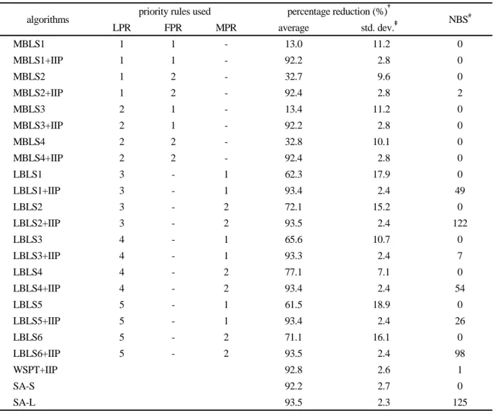
Table 1. Results of comparison with WSPT

algorithms priority rules used percentage reduction (%)

NBS

LPR FPR MPR average std. dev.

MBLS1 1 1 - 13.0 11.2 0

MBLS1+IIP 1 1 - 92.2 2.8 0

MBLS2 1 2 - 32.7 9.6 0

MBLS2+IIP 1 2 - 92.4 2.8 2

MBLS3 2 1 - 13.4 11.2 0

MBLS3+IIP 2 1 - 92.2 2.8 0

MBLS4 2 2 - 32.8 10.1 0

MBLS4+IIP 2 2 - 92.4 2.8 0

LBLS1 3 - 1 62.3 17.9 0

LBLS1+IIP 3 - 1 93.4 2.4 49

LBLS2 3 - 2 72.1 15.2 0

LBLS2+IIP 3 - 2 93.5 2.4 122

LBLS3 4 - 1 65.6 10.7 0

LBLS3+IIP 4 - 1 93.3 2.4 7

LBLS4 4 - 2 77.1 7.1 0

LBLS4+IIP 4 - 2 93.4 2.4 54

LBLS5 5 - 1 61.5 18.9 0

LBLS5+IIP 5 - 1 93.4 2.4 26

LBLS6 5 - 2 71.1 16.1 0

LBLS6+IIP 5 - 2 93.5 2.4 98

WSPT+IIP 92.8 2.6 1

SA-S 92.2 2.7 0

SA-L 93.5 2.3 125

†percentage reduction of the solutions of the algorithm from those obtained from the WSPT rule.

‡standard deviation.

# number of problems (out of 360 problems) for which the algorithm found the best solutions among those obtained from the heuristic algorithms included in the test.

time limit.

<Table I> shows performance (solution quality) of the al- gorithms tested in this research, four MBLS algorithms with and without IIP, six LBLS algorithms with and without IIP, the WSPT algorithm with and without IIP and two SA algorithms. Here, SA-S and SA-L denote the SA algorithms with shorter and longer CPU time limits, respectively. In general, the lot-based list scheduling algorithms worked better than the machine-based list scheduling algorithms. Among the lot-based list scheduling algorithms, LBLS2, LBLS4 and LBLS6, in which MPR2 is used, worked better than the other lot-based algorithms. Note that in MPR2, we determine the priority of a machine considering the number of alternative machines that can be used (without a record-dependent set- up) instead of the machine.

Solution values, the weighted sum of flowtimes of the wa-

fer lots, were reduced from those obtained from the WSPT rule by more than 60% with the lot-based list scheduling algorithms. The iterative improvement procedure (IIP) sig- nificantly improved initial schedules obtained from the list scheduling algorithms. Solution values from all algorithms with IIP were more than 90% smaller than those from the WSPT rule. In addition, the best solutions were obtained by algorithms with IIP in all problems but one, and the lot-based list scheduling algorithm with IIP gave the best solutions in all test problems except for four. When the improvement pro- cedure was used, solution quality was not affected very much by the initial schedules.

The iterative improvement procedure (IIP) was slightly more effective in improving a given solution than SA-S.

Note that the re-sequencing procedure used in IIP cannot be

easily implemented in the SA algorithms since the procedure

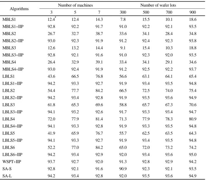
Table 2. Results for different numbers of machines and wafer lots

Algorithms Number of machines Number of wafer lots

3 5 7 300 500 700 900

MBLS1 12.4

12.4 14.3 7.8 15.5 10.1 18.6

MBLS1+IIP 92.8 92.2 91.7 91.0 92.2 92.1 93.5

MBLS2 26.7 32.7 38.7 33.6 34.1 28.4 34.8

MBLS2+IIP 93.0 92.3 91.9 91.2 92.4 92.3 93.8

MBLS3 12.6 13.2 14.4 9.1 15.4 10.3 18.8

MBLS3+IIP 92.8 92.1 91.6 91.0 92.3 92.0 93.5

MBLS4 26.4 32.9 39.1 33.4 34.1 29.1 34.6

MBLS4+IIP 93.0 92.4 91.9 91.2 92.5 92.2 93.7

LBLS1 43.6 66.5 76.8 56.6 63.1 64.1 65.4

LBLS1+IIP 94.2 93.3 92.7 91.9 93.4 93.5 94.8

LBLS2 54.4 77.7 84.2 66.5 72.5 74.0 75.4

LBLS2+IIP 94.2 93.4 92.8 91.9 93.5 93.6 94.9

LBLS3 61.8 65.3 69.6 58.8 65.7 67.3 70.6

LBLS3+IIP 94.1 93.2 92.6 91.7 93.3 93.4 94.7

LBLS4 72.0 77.9 81.4 71.3 77.9 78.3 80.9

LBLS4+IIP 94.1 93.3 92.8 91.9 93.3 93.5 94.8

LBLS5 41.9 65.9 76.7 55.7 62.5 63.5 64.3

LBLS5+IIP 94.1 93.3 92.7 91.9 93.4 93.5 94.8

LBLS6 52.2 77.0 84.2 65.0 72.0 73.2 74.2

LBLS6+IIP 94.2 93.4 92.9 92.0 93.4 93.6 95.0

WSPT+IIP 93.7 92.7 92.0 91.3 92.8 92.9 94.2

SA-S 92.8 92.1 91.6 90.9 92.3 92.1 93.5

SA-L 94.2 93.4 92.8 92.0 93.5 93.6 94.9

†percentage reduction of the solutions of the algorithm from those obtained from the WSPT rule

itself required relatively long time. Even though a much lon- ger CPU time is given to SA-L, in which the solution ob- tained from the best algorithm among the suggested algo- rithms was used as the initial solution, the solution could not be improved very much. Note that SA-L did not improve the initial schedules obtained from LBLS2+IIP in the test prob- lems except for three (In SA-L, the initial solution was ob- tained from LBLS2+IIP). This may be because the schedules obtained from LBLS2+IIP were very good already, and therefore, there was little room for improvement.

To see the performance of the algorithms on various prob- lem settings such as problem sizes and workloads, we per- formed another series of tests varying the numbers of ma- chines and wafer lots. <Table 2> shows results of this series of tests. The results are similar to those given in <Table 1>, which means that certain algorithms worked better than oth- ers regardless of problem settings. In addition, to see the ef- fect of the numbers of machines, wafer lots and wafer fami-

lies on the (relative) performance of the algorithms, an analy- sis of variance was done and results are given in <Table 3>.

From the results, one can see that the relative performance of the algorithms was affected by the problem settings. Note that, however, best performing algorithms consistently gave good results regardless of problem settings. Algorithms that did not work very well showed variance in their (relative) performance.

To see the differences in the performance of the algorithms,

we performed the Duncan’s multiple range test (Montgom-

ery, 2001). Results are given in <Table 4>. Note that per-

formance of algorithms included in the same group is statisti-

cally indifferent, while performance of algorithms in differ-

ent groups is different. The results show that the iterative im-

provement procedure (IIP) was very effective. There was no

statistically significant difference in the performance among

the algorithms with IIP, but these algorithms significantly

outperformed the algorithms without IIP. Without the IIP,

Table 3. Results of the analysis of variance

Source of variation Degrees of freedom Sum of squared error Mean squared error F

Algorithm (A) 22 237.622 10.801 1670.31

Number of wafer lots (W) 3 1.536 0.512 79.19

Number of families (F) 2 1.066 0.533 82.42

Number of machines (M) 2 2.159 1.079 167.01

A×W 66 0.691 0.010 1.61

A×F 44 3.508 0.079 12.33

A×M 44 10.031 0.228 35.26

Error 8096 52.352 0.006

Total 8279 308.967

Not) ^**There is difference in the effects at the significance level of 0.01.

Table 4. Results of Duncan’s multiple range test

algorithms APR

(%) Results (groups)

SA-L 93.5 A

LBLS2+IIP 93.5 A

LBLS6+IIP 93.5 A

LBLS4+IIP 93.4 A

LBLS1+IIP 93.4 A

LBLS5+IIP 93.4 A

LBLS3+IIP 93.3 A

WSPT+IIP 92.8 A

MBLS4+IIP 92.4 A

MBLS2+IIP 92.4 A

MBLS1+IIP 92.2 A

MBLS3+IIP 92.2 A

SA-S 92.2 A

LBLS4 77.1 B

LBLS2 72.1 C

LBLS6 71.1 C

LBLS3 65.6 D

LBLS1 62.3 F

LBLS5 61.5 F

MBLS4 32.8 G

MBLS2 32.7 G

MBLS3 13.4 H

MBLS1 13.0 H

WSPT 0.0 I

†average percentage reduction.

performance of the lot-based algorithms was significantly better than that of the machine-based algorithms and the WSPT algorithm, which is currently used in practice.

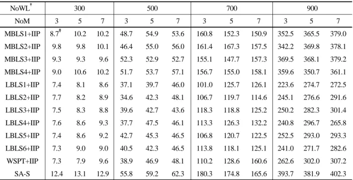
The performance of the algorithms in terms of computation time is shown in <Table 5>. Computation times required for the WSPT rule and the list scheduling algorithms without IIP are not

shown in the table, since they were very short (a solution was ob-

tained within a fraction of a second). The computation time was

more affected by the number of wafer lots than by the number of

machines, possibly because the number of alternatives to be con-

sidered for re-assignment as well as re-sequencing increases

more quickly as the number of wafer lots increases than as the

Table 5. Computation time required for each problem

NoWL

300 500 700 900

NoM 3 5 7 3 5 7 3 5 7 3 5 7

MBLS1+IIP 8.7

10.2 10.2 48.7 54.9 53.6 160.8 152.3 150.9 352.5 365.5 379.0 MBLS2+IIP 9.8 9.8 10.1 46.4 55.0 56.0 161.4 167.3 157.5 342.2 369.8 378.1 MBLS3+IIP 9.3 9.3 9.6 52.3 52.9 52.7 155.1 147.7 157.3 369.5 368.1 379.2 MBLS4+IIP 9.0 10.6 10.2 51.7 53.7 57.1 156.7 155.0 158.1 359.6 350.7 361.1

LBLS1+IIP 7.4 8.1 8.6 37.1 39.7 46.0 101.0 125.7 126.1 223.6 274.7 272.5 LBLS2+IIP 7.7 8.2 8.9 34.6 42.3 48.1 106.7 119.7 114.6 245.1 276.6 291.6 LBLS3+IIP 7.5 8.3 8.8 39.6 42.7 43.6 118.3 118.8 125.2 250.2 282.3 301.4 LBLS4+IIP 7.6 8.6 9.3 37.7 47.5 46.1 113.3 126.3 132.2 240.8 296.7 265.8 LBLS5+IIP 7.4 8.6 9.2 42.7 45.3 46.5 106.8 120.7 122.5 252.5 293.0 293.3 LBLS6+IIP 7.3 9.0 9.0 40.5 42.3 46.5 113.8 118.1 125.1 241.0 271.7 282.6

WSPT+IIP 7.3 7.9 9.6 38.9 46.9 48.1 110.2 128.6 160.6 262.6 302.0 307.2 SA-S 12.4 13.1 12.9 55.8 59.2 62.3 180.3 174.8 165.6 393.7 381.9 402.3

†NoWL and NoM stand for the number of wafer lots and the number of machines, respectively.

‡Average of CPU seconds.

number of machines increases. Since problems with the largest size could be solved in less than 10 minutes, the algorithms with IIP can also be used for practical problems in many cases.

One may need to select an algorithm for the deposition workstation considering not only the quality of schedules and CPU time required but also how the scheduling algorithm for the deposition workstation is used. If a long time can be given for the scheduling decision, one may include IIP in the schedul- ing algorithm. However, IIP cannot be used if the problem should be solved in a very short time. For instance, if schedul- ing decisions are to be made on a real-time basis (in a real-time scheduling system), or the scheduling problem at the deposition workstation should be solved many times to obtain a schedule for the overall fab (in a scheduling system for the overall fab), the scheduling problem should be solved in a very short time, and the lot-based list scheduling algorithms without IIP may be very useful in such circumstances. Note that a schedule for the deposition workstation should be synchronized with those for other workstations in the fab. In such circumstances, 10 mi- nutes for one workstation is not short enough, since the data used for scheduling at the deposition workstation (such as ready times of lots) depend on schedules of other workstations, and at the same time, data for scheduling at other workstations depend on schedules at the deposition workstation.

4. Concluding Remarks

This study focuses on the problem of scheduling wafer lots in the deposition workstation in a semiconductor wafer fab-

rication facility. There are multiple identical machines in the deposition workstation, and there are two types of setups (record-dependent setup and family setup) required at the deposition machines. We suggested two-phase heuristic algo- rithms in which priority-rule-based list scheduling algorithms were used to generate initial schedules in the first phase and the schedule was improved in the second phase. Results of computational tests on randomly generated test problems showed that the suggested algorithms (with and without the improvement procedure of the second phase) outperformed a scheduling method used in a real manufacturing system in terms of the sum of weighted flowtimes of the wafer lots.

Also, the improvement procedure was very effective in re- ducing the solution values.

This research can be extended in several directions. For example, since the system considered here is a subsystem of a larger system with complicated material flows, it may be necessary to devise a scheduling method that can deal with the whole system. If the subsystem is a bottleneck of the whole system (it was actually a bottleneck in the system con- sidered here at the time this research was conducted), we can use the approach suggested in the research of Lee et al.

(2004), in which a schedule for a bottleneck stage is con-

structed first and then schedules for upstream stages are con-

structed backward and those for downstream stages are con-

structed forward based on the schedule for the bottleneck. In

addition, if the heuristic algorithms suggested in this research

are modified appropriately, they can be used for other ob-

jectives such as minimizing tardiness or makespan, since

general approach used in this research can be easily adapted

to various scheduling problems.

References

Allahverdi, A., Ng, C T., Cheng, T. C. E., and Kovalyov, M. Y. (2008), A survey of scheduling problems with setup times and costs, European Journal of Operational Research, 187(3), 985-1032.

Arzi, Y. and Raviv, D. (1998), Dispatching in a workstation belonging to a re-entrant production line under sequence-dependent set-up times, Production Planning and Control, 9(7), 690-699.

Azizoglu, M. and Kirca, O. (1999), On the minimization of total weight- ed flow time with identical and uniform parallel machine, European Journal of Operational Research, 113(1), 91-100.

Azizoglu, M. and Webster, S. (2003), Scheduling parallel machines to minimize weighted flowtime with family set-up times, International Journal of Production Research, 41(6), 1199-1215.

Barnes, J. and Brennan, J. J. (1977), An improved algorithm for schedul- ing jobs on identical machines, AIIE Transactions on Computing,

Bruno, J., Coffman, J. E., and Sethi, R. (1974), Scheduling independent tasks to reduce mean finishing time, Communications of ACM, 17(7), 382-387.

Chern, C. C. and Liu, Y. L. (2003), Family-based scheduling rules of a sequence-dependent wafer fabrication system, IEEE Transactions on Semiconductor Manufacturing, 16(1), 15-25.

Cigolini, R., Comi, A., Micheletti, A., Perona, M., and Portioli, A. (1999), Implementing new dispatching rules at SGS-Thomson Microele- ctronics, Production Planning and Control, 10(1), 97-106.

Dessouky, M. M. (1998), Scheduling identical jobs with unequal ready times on uniform parallel machines to minimize the maximum late- ness, Computers and Industrial Engineering, 34(4), 794-806.

Dunstall, S. and Wirth, A. (2005a), A comparison of branch-and-bound algorithms for a family scheduling problem with identical parallel ma- chines, European Journal of Operational Research, 167(2), 283-296.

Dunstall, S. and Wirth, A. (2005b), Heuristic methods for the identical parallel machine flowtime problem with set-up times, Computers and Operations Research, 32(9), 2479-2491.

Duenyas, I., Fowler, J. W., and Schruben, L. W. (1994), Planning and scheduling in Japanese semiconductor manufacturing, Journal of Manufacturing Systems, 13(5), 323-332.

Eastman, W., Even, S., and Isaacs, I. (1964), Bounds for the optimal scheduling of n jobs on m processors, Management Science, 11(2), 268-279.

Elmaghraby, S. E. and Park, S. H. (1974), Scheduling jobs on a number of identical machines, AIIE Transactions on Computing, 6(1), 1-13.

Fowler, J., Hogg, G. L., and Phillips, D. T. (1992), Control of multi- porduct bulk service diffusion/oxidation processes, IIE Transactions

Fowler, J., Knutson, K., and Carlyle, M. (2000), Comparison and evalua- tion of lot-to-order matching policies for a semiconductor assembly and test facility, International Journal of Production Research, 38(8), 1841-1853.

Glassey, C. R. and Resende, M. C. G. (1988), A scheduling rule for job release in semiconductor fabrication, Operations Research Letters,

Glassey, C. R. and Weng, W. W. (1991), Dynamic batching heuristic for simultaneous processing, IEEE Transactions on Semiconductor Manufacturing, 4(2), 77-82.

Graves, S. C., Meal, H. C., Stefek, D., and Zeghmi, A. H. (1983), Scheduling of re-entrant flow shops, Journal of Operations

Management, 3(4), 197-207.

Johri, P. K. (1993), Practical issues in scheduling and dispatching in semiconductor wafer fabrication, Journal of Manufacturing systems,

Kim, Y.-D., Kim, J.-U., Lim, S.-K., and Jun, H.-B. (1998a), Due-date based scheduling and control policies in a multiproduct semi- conductor wafer fabrication facility, IEEE Transactions on Semiconductor Manufacturing, 11(1), 155-164.

Kim, Y-D., Lee, D-H., and Kim, J-U. (1998b), A simulation study on lot release control, mask scheduling, and batch scheduling in semi- conductor wafer fabrication facilities, Journal of Manufacturing Systems, 17(2), 107-117.

Ko, H. H., Baek, J. K., Kang, Y. H., and Kim, S. S. (2004), A scheduling scheme for restricted parallel machines cycling process, Journal of the Korean Institute of Industrial Engineers, 30(2), 107-119.

Lawler, E. L. and Moore, J. M. (1969), A functional equation and its ap- plication to resource allocation and sequencing problems, Manage- ment Science, 16(1), 77-84.

Lee, C. Y. and Uzsoy, R. (1992), A new dynamic programming algo- rithm for the parallel machines total weighed completion time prob- lem, Operational Research Letters, 11(2), 73-75.

Lee, G.-C., Kim, Y.-D., and Choi, S.-W. (2004), Bottleneck-focused scheduling for a hybrid flowshop, International Journal of Produc- tion Research, 42(1), 165-181.

Lee, K. H., Hong, Y. S., and Kim, S. Y. (1995), Production scheduling semiconductor wafer fabrication process, Journal of the Korean Institute of Industrial Engineers, 21(3), 357-369.

Lin, J. T., Wang, F. K., and Kuo, P. C. (2005), A parameterized- dispatch- ing rule for a logic IC sort in a wafer fabrication, Production Planning and Control, 16(5), 426-436.

Lou, S. X. C. and Karger, P. W. (1989), A robust production control poli- cy for VLSI wafer fabrication, IEEE Transactions on Semiconductor Manufacturing, 2(4), 159-164.

Monch, L., Balasubramanian, H., Fowler, J. W., and Pfund, M. E. (2005), Heuristic scheduling of jobs on parallel batch machines with in- compatible job families and unequal ready times, Computers and Operations Research, 32(11), 2731-2750.

Monma, C. L. and Potts, C. N. (1989), On the complexity of scheduling with batch setup times, Operational Research, 37(5), 798-804.

Montgomery, D. C. (2001), Design and analysis of experiments, Wiley, New York.

Min, H. S. and Yih, Y. (2003), Selection of dispatching rules on multiple dispatching decision points in real-time scheduling of a semi- conductor wafer fabrication system, International Journal of Produc- tion Research, 41(16), 3932-3941.

Nawaz, M., Enscore, E. E., and Ham, I. (1983), A heuristic algorithm for the m-machine, n-job flow-shop scheduling problem, Omega, 11(1), 91-95.

Park, M.-W. and Kim, Y.-D. (1997), Search heuristics for a parallel ma- chine scheduling problem with ready times and due dates, Computers and Industrial Engineering, 33(3-4), 793-796.

Pfund, M., Fowler, J. W., Gadkari, A., and Chen, Y. (2008), Scheduling jobs on parallel machines with setup times and ready times, Compu- ters and Industrial Engineering, 54(4), 764-782.

Robinson, J. K., Fowler, J. W., and Bard, J. F. (1995), Use of upstream and downstream information in scheduling semiconductor batch op- erations, International Journal of Production Research, 33(7), 1849-1869.

Schutten, J. M. J. and Leussink, R. A. M. (1996), Parallel machine sched-

uling with release dates, due dates and family setup times, Interna- tional Journal of Production Economics, 46/47, 119-125.

Uzsoy, R., Lee, C. Y., and Martian-Vega, L. A. (1992), A review of pro- duction planning and scheduling models in the semiconductor in- dustry Part I : System characteristics, performance evaluation and pro- duction planning, IIE Transaction, 24(4), 47-60.

Uzsoy, R., Lee, C. Y., and Martian-Vega, L. A. (1994), A review of pro- duction planning and scheduling models in the semiconductor in- dustry Part II : Shop-floor control, IIE Transaction, 26(5), 44-55.

Webster, S. (1993), A priority rule for minimizing weighted flow time in a class of parallel machine scheduling problems, European Journal of Operational Research, 70(3), 327-334.

Webster, S. (1994), A note on “schedule of n jobs on two identical ma-

chines to minimize weighted mean flow time, Computers and Industrial Engineering, 26(4), 795-796.

Webster, S. and Azizoglu, M. (2001), Dynamic programming algo- rithms for scheduling parallel machines with family setup times, Computers and Operations Research, 28(2), 127-137.

Wein, L. M. (1988), Scheduling semiconductor wafer fabrication, IEEE Transactions on Semiconductor Manufacturing, 1(3), 115-130.

Yoon, H. J. and Lee, D. Y. (2004), Deadlock-free scheduling of photo- lithography equipment in semiconductor fabrication, IEEE Transa- ctions on Semiconductor Manufacturing, 17(1), 42-54.

Zhu, X., Wilhelm, W. E. (2006), Scheduling and lot sizing with sequ-

ence-dependent setup : a literature review, IIE Transactions, 38(11),

987-1007.