General Circulation Model Derived Climate Change Impact and Uncertainty Analysis of Maize Yield in Zimbabwe

(1)

DOI:http://dx.doi.org/10.5389/KSAE.2012.54.4.083

General Circulation Model Derived Climate Change Impact and Uncertainty Analysis of Maize Yield in Zimbabwe

GCM 예측자료를 이용한 기후변화가 짐바브웨 옥수수 생산에 미치는 영향 및 불확실성 분석

Nkomozepi, Temba D^*

․Chung, Sang-Ok

^*,†

은코모제피 템바․정상옥

ABSTRACT

짐바브웨는 식량부족을 격어 오고 있으며, 이는 기후변화에 따른 수자원의 부족, 인구증가, 개발 및 환경보전 등으로 인하여 앞으로는 더욱 심화될 것으로 보인다. 3가지 배출시나리오 (A2, A1B, B1)에 대한 13개의 GCM 기후자료로부터 상세화한 기후예측값과 AquaCrop 작물모형을 이용하여 기후변화가 짐바브웨의 주곡인 옥수수의 수확량에 미치는 영향과 모형예측값의 불확실성을 분석하였다. 작물생육환 경이 잘 유지된다고 가정하고 옥수수 잠재생산량을 모의한 결과 기준년도 (1970s)에 비해 2020s, 2050s and 2090s 년대에 평균 (범위) 8 % (6-9 %), 14 % (10-15 %) 및 16 % (11-17 %) 증가할 것으로 예측되었다. 같은 기간에 대한 물의 생산성은 평균 (범위) 7 % (4-13 %), 13 % (6-30 %) 및 15% (6-23 %) 증가할 것으로 예측되었다. 기온의 꾸준한 상승과 대기중 이산화탄소 농도 증가로 인한 시비효과로 인하여 미래에는 옥수수 단위 생산량과 물의 생산성이 증가할 것으로 예측되었으며 증가 범위를 보면 모형간의 변동성이 상 당히 큰 것을 알 수 있었다. 본 연구결과는 기후변화가 짐바브웨의 옥수수 생산량에 미치는 영향과 변동성을 제시하므로서 장기적인 식 량계획의 기초자료로 이용될 수 있을 것이다.

Keywords: General circulation model; yield; Zimbabwe; maize; climate change; uncertainty

I. INTRODUCTION

^*

Southern Africa is subject to recurrent food shortages which could worsen as future water scarcity is inevitable due to increasing population demand for food, development and environmental maintenance (Cane et al., 1994; Nyakudya and Stroosnijder, 2011). Climate change on the other hand is expected to increase climate variability and exert more pressure on food security in Zimbabwe (Zinyengere et al., 2011). The sensitivity of southern Africa to climatic extremes is compounded by the strong dependence upon agriculture, high population growth rate and unstable economic conditions.

Crop yield forecasting with sufficient lead time is critical to support food security planning.

* Department of Agricultural Engineering, Kyungpook National University

† Corresponding author Tel.: +82-53-950-5734 Fax: +82-53-950-6752

E-mail: [email protected] 2012년 4월 13일 투고 2012년 6월 13일 심사완료 2012년 6월 14일 게재확정

In Zimbabwe, previous seasonal crop forecasts were indirectly inferred from El Niño Southern Oscillation based climate forecasting (Cane et al., 1992; Taylor et al., 2002).

Soil moisture stress is also a primary determinant of crop yield and rainfall estimates are the most used inferential tool for predicting seasonal crop yields in Zimbabwe (Manatsa et al., 2011). Recent studies have incorporated the use of crop simulation models, remote sensing and geospatial analysis to capture the relationship between yields and other variables such as temperature, humidity, radiation etc. during the growing season (Chung, 2010;

Nkomozepi and Chung, 2011b; Zinyengere et al., 2011;

Manatsa et al., 2011). In Korea, several studies have been done on climate change impact on evapotranspiration (ET) and paddy irrigation requirement (e.g., Chung, 2009; Hong et al., 2009; Yoo et al., 2012).

In order for a study based on the potential impacts of climate change on long term maize yields to be implemen- table, the relevant constraints have to be surmounted. Water shortages and heat stress are two of the most important environmental factors limiting crop growth, development,

(2)

and yield (Harrison et al., 2011). High temperatures and low soil moisture during the flowering stage are especially harmful as they can inhibit successful formation of kernels through compromising pollen viability. Whether these losses are realized will depend on the effectiveness of adaptation strategies, which include shifts in sowing dates, switches to longer maturing varieties, and the development of new varieties that can better withstand water and heat stress and better utilize elevated atmospheric carbon dioxide (CO2) concentration.

The complexity of the ecosystem results in responses to changes in external forcing that can vary from subtle to chaotic. The sensitivity of the earth system to anthropogenic greenhouse gas emissions associated with nonlinearity can lead to distortion and/or misinterpretation of climate change signals thereby reducing the usefulness of seasonal climate forecasts that use single climate prediction models.

The impacts of climate change on crop productivity are often assessed using data from general circulation models (GCMs) as an input to crop simulation models. Climate change involves shifts in both mean and variability of climate parameters, and experimental results and simulations have shown same-order effects on crop growth and yield.

It is therefore important for impact models to be able to capture the uncertainty associated with yield projections (Holzkämper et al., 2012).

Because any mathematical model is a simplification or approximation of reality, there is inevitable uncertainty.

Yao et al. (2011) summarized five types of uncertainty namely context uncertainty, input uncertainty, model structure uncertainty, parameter uncertainty and modeling technical uncertainty. There is also large uncertainty in the simulation and assessment of climate change affecting agriculture in terms of the climate prediction, crop models and integrating climate models with crop models, and the uncertainty propagates through the assessment process (Nkomozepi and Chung, 2012).

The purpose of this study is to generate climate scenarios from multiple GCMs, simulate multiple maize yield forecasts and assess them for uncertainty. AquaCrop crop model was chosen in this study because the model can use few parameters while maintaining accuracy making it attractive for locations where some information may be unavailable.

AquaCrop is a dynamic process-based crop model that resolves plant and environmental processes relevant to crop growth and is rooted in physical responses dependent on developmental stage and crop stresses that may interact in a non-linear manner.

II. MATERIAL AND METHODS

1. Study Area

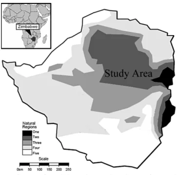
Agriculture in Zimbabwe is spread across five natural agro-ecological zones that range from areas of high rainfall and productivity in the north to areas of extremely low productivity where rainfall is sparse and variable in the south. This study was conducted on 3 provinces mostly situated in natural agro-ecological region II (NR II), located in the north-eastern part of the Zimbabwe (Fig. 1). Kutsaga Research Station in Harare city (17° 56' S, 31° 05' E;

1,479 m above mean sea level) was selected for this study to reflect typical farm management practices under commercial production conditions for NR II. Kutsaga station was established in 1994 and has been used in related studies that consider irrigation and drainage for NR II (Savva and Frenken, 2002). In addition, homogeneous areas

Fig. 1 Map of Zimbabwe showing boundaries of natural regions and the study area (NR II)

(3)

Table 1 Description of natural agro-ecological region II (FAO, 2006)

Land use sector Area (1,000 ha) (%)

Population (1,000) (%)

Maize area (1,000 ha) (%) Large-scale commercial farming 2,422 (41.3) 410 (11.0) 145 (12.2) Small-scale commercial farming 1,893 (32.3) 988 (26.5) 503 (42.5) Communal areas 926 (15.8) 2,063 (55.4) 532 (44.9) Parks and urban areas 620 (10.6) 262 (7.1) 5 (0.4)

Total 5,861 (100) 3,723 (100) 1,185 (100)

with more intensive management, modern cultivars, and heavy use of mechanical equipment are more suited to crop model simulations based upon a single representative site (Ruane et al., 2011).

The 5,861,400 ha study area is covered by a mixture of ferric and gleyic luvisols which are loamy with heavier textured sub-soils which are inherently fertile (FAO, 2006).

NR II is situated in the hilly and mountainous northern part of the country with valleys that are used for agriculture and mining. The altitude ranges from 900 to 1,500 m above sea level. Approximately 74 % of the study area is utilized for commercial agriculture to produce maize, soybeans, cotton, wheat, groundnuts, tobacco and horticultural crops such as roses, cut flowers and vegetables. The remaining 25 % consists of communal areas, national parks and urban settlements (Table 1). 47 % and 7 % of the maize grown in the large scale (LSCF) and small scale commercial (SSCF) and farming sectors respectively is under full or partial control irrigation. Maize grown in the communal areas is rain-fed and under subsistence farming. The study region has a sub-tropical climate and has fairly reliable rainfall which ranges from 750 to 1,000 mm per year and falls from November to April. Maize (Zea mays) crop was selected to be investigated since it is the main crop in this area and a range of 3 future climate periods to be relevant to planning of agricultural infrastructure and policy. The maize is planted in late October and harvested in late March.

2. Climate and Yield Data

Historical climate and official post-harvest yield data were provided by the Central Statistical Office of Zimbabwe and FAOSTAT (www.faostat.com). Future climate data for Kutsaga station were from the IPCC 4^th assessment report

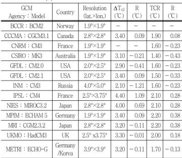
and were downloaded from the IPCC Data Distribution Center (http://www.ipcc-data.org) for the periods of 2011 -2030 (2020s), 2046-2065 (2050s) and 2080-2099 (2090s) for the 13 GCMs used in this study (Table 2). 30 year mean monthly values were adopted to eliminate natural inter-annual to inter-decadal variability. GCMs are systems of partial differential equations based on the basic laws of physics, fluid motion, and chemistry. The outputs include temperature and precipitation estimates across the grid, as well as many other variables. The boundary conditions include emissions of atmospheric gases (including CO2) and volcanic eruptions (Fildes and Kourentzes, 2011).

The different capabilities and limitations of the GCMs give rise to output variability (uncertainty) as shown by the equilibrium climate sensitivity (ΔTx2), transient climate response (TCR), and residual or fitting error (R) (Table 2).

Model outputs from INM：CM3, IPSL：CM4 and MIROC3.2 were flagged as outliers based on the interquartile range method but were not excluded from this study because we do not assume a normal distribution. Uncertainty can be further attributed to the different discretization, para- meterization and carbon cycle models used by the GCM (Chung and Nkomozepi, 2012). Uncertainty introduced by GCM projections reflects the state of agreement across models, but it is possible that future conditions fall outside

Table 2 GCM description with equilibrium climate sensitivity (ΔTx2), transient climate response (TCR), and residual error (R)

GCM

Agency：Model Country Resolution (lat.×lon.)

ΔTx2

(℃) R (℃)

TCR (℃)

R (℃)

BCCR：BCM2 Norway 1.9°×1.9° －－－－

CCCMA：CGCM3.1 Canada 2.8°×2.8° 3.40 0.09 1.90 0.08 CNRM：CM3 France 1.9°×1.9° －－ 1.60 －0.23 CSIRO：MK3 Australia 1.9°×1.9° 3.10 －0.21 1.40 －0.43 GFDL：CM2.0 USA 2.0°×2.5° 2.90 －0.41 1.60 －0.23 GFDL：CM2.1 USA 2.0°×2.5° 3.40 0.09 1.50 －0.33 INM ：CM3 Russia 4.0°×5.0° 2.10 －1.21 1.60 －0.23 IPSL：CM4 France 2.5°×3.75° 4.40 1.09 2.10 0.28 NIES：MIROC3.2 Japan 2.8°×2.8° 4.00 0.69 2.10 0.28 MPIM：ECHAM 5 Germany 1.9°×1.9° 3.40 0.09 2.20 0.38 MRI：CGM2.3.2 Japan 2.8°×2.8° 3.20 －0.11 2.20 0.38 UKMO：HadCM3 UK 2.5° x3.75° 3.30 －0.01 2.00 0.18

METRI：ECHO-G Germany

/Korea 3.9°×3.9° 3.20 －0.11 1.70 －0.13

(4)

of this projected range and each new climate simulation requires a costly new impacts assessment. An alternative approach (used herein) would be to use a crop model to simulate the yield responses to a broader range of climate states or scenarios, capturing a wider uncertainty space for integrated assessment models. Climate projections for the B1, A1B, and A2 scenarios of the IPCC Special Report on Emissions Scenarios (SRES) were used in this study.

The mean annual atmospheric CO2 concentration is estimated to reach 856, 717 and 549 ppm by 2100 for the A2, A1B and B1 scenarios respectively. The existence of SRES scenarios merely serves as a reminder that these estimates of future climates are imprecise; they are the output of models striving to represent complex natural systems.

While it is ideal to use observed records for the baseline, suitable data were not readily available and this study relied on an International Water Management Institute (IWMI) modeled dataset with a spatial resolution of 10 minutes-Arc (New et al., 2002). The IWMI database is currently the most extensive global climate database in terms of resolution, coverage and number of parameters that is available in the public domain (Droogers and Allen, 2002). The monthly average dataset was developed using observations from about 56,000 stations around the world from 1961 to 1990 in which Zimbabwe is well represented.

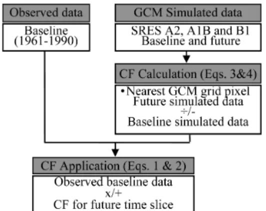
The change factor (CF) procedure was used as in Chung and Nkomozepi (2012). Key advantages of the CF approach are the ease and speed of application and the direct scaling of the scenario in line with changes suggested by the GCM or RCM. The procedure involves 3 steps (Fig. 2). The

Fig. 2 Flowchart of the CF method (modified from Nkomozepi and Chung, 2011a)

first step involves the establishment of long term baseline climatology data (1961-1990). In the second step, the change factors in the equivalent variable are calculated for the GCM grid box closest to the target site. In the third step, the change factor obtained from the GCM projections for a particular time slice and a SRES scenario is applied to each monthly average in the baseline. Absolute change factors were used for temperature and relative changes for rainfall, wind speed and radiation. This process is shown by the following equations:

Tm,fut＝TIWMI,m,1975s＋∆Tfut (1)

Pm,fut＝PIWMI,m,1975s＋∆Pfut (2)

where Tm,fut and Pm,fut are the temperature and other weather parameters (rainfall, wind speed or radiation) for month m in the future period, TIWMI,m,1975s and PIWMI,m,1975s are observed temperature and other weather parameters for month m for the 1975s (baseline period), ∆Tfut and ∆Pfut are the long term change factors of monthly average temperature and other weather parameters and are calculated as follows;

∆Tfut＝TGCM,m,fut－TGCM,m,1975s (3)

∆Pfut＝PGCM,m,fut÷PGCM,m,1975s (4)

where TGCM,m,1975s, PGCM,m,1975s, TGCM,m,fut and PGCM,m,fut are the long term (20 year) monthly means for month m in the baseline and future periods simulated by GCM for a given scenario.

3. AquaCrop Model

When forecasting crop yields, simplified descriptions of reality such as homogenous crop fields with defined thematic boundaries, internal characteristics and external driving variables with an apparent absence of uncertainty are generally used (Nkomozepi and Chung, 2011b). AquaCrop model has a structure that overarches the soil-plant- atmosphere continuum. It includes the soil, with its water balance; the plant, with its development, growth and yield processes; and the atmosphere, with its thermal regime,

(5)

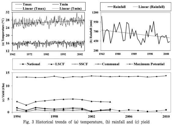
Fig. 3 Historical trends of (a) temperature, (b) rainfall and (c) yield rainfall, irrigation, evaporative demand and carbon dioxide

concentration. Additionally, some management aspects are explicitly considered, as they will affect the soil water balance, crop development and therefore crop yield. The functional relationships between the different model com- ponents and detailed descriptions can be found in Raes et al. (2010).

Due to model and data limitations, effects of pests and diseases, availability of water for irrigation, availability of nutrients, socio-economic factors and possible changes in crop sowing-maturity duration (calendar day used) in the future were not considered (i.e. potential yield). Crop response was simulated under irrigation for the baseline and future scenarios. The maximum potential yield was simulated for the baseline, 1962-2010 and future periods using AquaCrop. The maximum potential yield will be used in the quantification of the uncertainty of the potential impacts of climate change on maize yields.

III. RESULTS AND DISCUSSION 1. Historical Climate and Yield

The maximum and minimum temperatures, yield (1994-

2010) and rainfall from 1962 to 2010 are shown in Fig. 3 (a), (b) and (c). Over the 48 year period, the maximum temperatures showed a higher increasing trend than minimum temperature. In spite of the increases in temperature, the diurnal temperature variations lie within the limits for optimum maize growth. The large-scale commercial farming (LSCF) and maximum potential yields showed an increasing trend while the small-scale commercial farming (SSCF), communal and the national average yields showed a declining trend. Linear regression showed R² values of 0.23, 0.50, and 0.3 for the communal, SSCF and national average yields respectively. The actual yields realized by the different sectors within the study area are significantly less than the simulated maximum potential values (about 13 t ha^－1) and research trials yields.

The discrepancy can be accounted for by classifying maize yield into maximum potential, attainable and actual yield.

The maximum potential yield is influenced by CO2, solar radiation, temperature and crop features. The attainable yield is a fraction of the potential yield as influenced by limiting factors such as water and nutrient availability. The actual yield refers to the fraction of attainable yield as influenced by reducing management factors such as weeds, pests and diseases. In Zimbabwe, the actual yields are further affected

(6)

Fig. 5 Box and whisker plots for relative changes in WP and yield by inaccessibility to capital, poor quality seeds and the

non-use of climate information. The socioeconomic and political factors which are beyond the scope of neither climate change nor this study including the changing of land ownership in Zimbabwe complicate the relationship between crop yields and the climatic factors. The observed yields (Fig. 3(c)) show that LSCF has much higher values than the others. This is mainly because of LSCF manages water, weeds and pests much better than the others.

The IPCC climate projections for the study area suggest average annual temperature increases of 1.1 ℃, 2.3 ℃ and 3.6 ℃ from the baseline of 21.4 ℃ for the 2020s, 2050s and 2090s respectively. Changes in annual effective rainfall were projected to range from －16 to ＋9 %, － 19 to 8 % and －16 to 7 % from the baseline of 510 mm for the 2020s, 2050s and 2090s respectively.

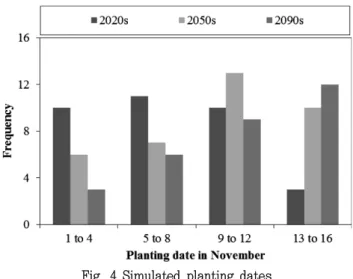
2. Planting Dates

The simulated planting date for the baseline was 4 November and lies within the normal range determined by the Agricultural Research and Extension Services and Meteorological Services Department methods in Raes et al.

(2004). The onset of the growing season was generated for each scenario based on climatic criteria. The onset of the season is preceded by at least 30 mm of cumulative rainfall from the start of the rainy season. The planting dates for the future were recorded into classes of four days from the

Fig. 4 Simulated planting dates

1^st to the 16^th of November (Fig. 4). The planting date distribution shifted torwards the right because of the decreased rainfall in October and November.

3. Maize Yield and Water Productivity

The characteristics of individual distributions of projections are summarized by graphical and tabular forms. In the box and whisker plots, the length of the box in the plot is a measure of the variability of the distribution; it shows the middle 50 % of the distribution (interquartile range). The lines in the middle of the boxes represent the median while the error bars denote upper and lower limits of the data.

The simulated changes of the maize yield (t ha^－1) and

(7)

water productivity (WP) (kg m^－3) from the baseline values are shown in Fig. 5. The yields are predicted to be significantly lower in the B1 scenario and increasing in the future for all scenarios. The 2050s B1 scenario showed the most variable simulated yield changes and the B1 scenario had the highest range in all the time slices.

The respective medians of the WP also show increasing trends for the future. The increased WP can be attributed to that although maize is a C4 plant, the changes initiated by increase in atmospheric CO2 concentration following precise signal transduction pathway maize will lead to increased photosynthesis and reduced stomatal conductance.

Table 3 and 4 show the simulated changes of the maize yield (t ha^－1) and WP (kg m^－3) from the baseline values.

The yield increases in the future periods and was projected to reach the highest in the 2090s A2. The increases in yield can be attributed to the expected increase in the atmospheric CO2 concentration. CO2 concentration can affect both the growth and water use of many plants through its first-order effect on photosynthesis and transpiration. As well as having direct effects on vegetation and biomass, it is also the major greenhouse gas associated with global climate change. Maize yields were simulated to increase by an average (and range) of 8 % (6-9 %), 14 % (10-15 %) and 16 % (11-17 %) in 2020s, 2050s and 2090s respectively.

Table 3 Projected change of potential maize yield from the baseline (%)

GCM 2020s 2050s 2090s

A2 A1B B1 A2 A1B B1 A2 A1B B1

BCM2 - 7.3 6.5 - 13.2 10.5 - 16.4 13.5

CGCM - 9.0 - - 15.3 - - 16.1 -

CNRM：CM3 7.6 7.8 - 14.7 14.7 - 16.9 16.4 - MK3 7.0 6.8 6.1 12.2 12.2 10.1 17.0 16.1 10.9 GFDL2.0 8.1 8.2 7.4 14.3 15.2 11.9 16.4 16.2 13.4 GFDL：CM2.1 8.1 8.0 7.4 15.1 15.0 12.4 16.8 16.0 13.4 INM：CM3 8.3 9.0 9.3 15.2 15.2 12.8 17.1 16.3 14.3 IPSL：CM4 7.8 8.2 7.8 15.3 15.3 13.1 17.1 16.0 14.1 MIROC3.2 9.1 7.4 7.2 14.9 14.3 12.2 17.2 16.6 14.3 ECHAM 5 7.9 7.6 7.7 15.2 15.1 13.5 16.9 16.2 13.9 CGM2.3.2 7.2 6.8 6.8 14.2 13.9 11.0 17.3 16.4 13.8 HadCM3 7.5 7.8 7.0 14.9 14.8 13.0 16.8 16.2 14.0 ECHO-G 7.6 7.5 - 14.3 14.8 - 17.1 16.5 - Average (Range) 8 (6-9) 14 (10-15) 16 (11-17)

*Baseline value; 12.9 t ha^－1

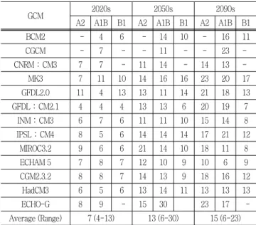
The WP was also projected to increase by an average (and range) of 7 % (4-13 %), 13 % (6-30 %) and 15 % (6-23 %) in 2020s, 2050s and 2090s respectively.

Table 5 shows the average (and range) simulated evaporation (Ea) and transpiration (Ta). The transpiration values are generally on a slight increasing trend for all three time slices with a few models that are outliers as shown by the ranges in Table 5. Evaporation was simulated to gradually increase over the future periods at a higher rate than the transpiration and had higher variability (uncertainty). The higher uncertainty in evaporation values shows that evaporation will be more affected by the future climate change. The planting date proved to significantly alter the simulated ET.

This is because the simulated reference ET (ETo) in the

Table 4 Projected change of maize WP from the baseline (%)

GCM 2020s 2050s 2090s

A2 A1B B1 A2 A1B B1 A2 A1B B1

BCM2 - 4 6 - 14 10 - 16 11

CGCM - 7 - - 11 - - 23 -

CNRM：CM3 7 7 - 11 14 - 14 13 -

MK3 7 11 10 14 16 16 23 20 17

GFDL2.0 11 4 13 13 11 14 21 18 13

GFDL：CM2.1 4 4 4 13 13 6 20 19 7

INM：CM3 6 7 6 11 11 10 15 14 8

IPSL：CM4 8 5 6 14 14 14 17 21 12

MIROC3.2 9 6 6 21 14 10 18 11 8

ECHAM 5 7 8 7 12 10 9 10 6 9

CGM2.3.2 8 8 7 14 13 9 18 16 12

HadCM3 6 5 6 13 14 11 13 13 13

ECHO-G 8 9 - 15 30 23 17 -

Average (Range) 7 (4-13) 13 (6-30) 15 (6-23)

*Baseline value; 2.7 kg m^－3

Table 5 AquaCrop simulated Ea and Ta for 3 SRES scenarios and 13 GCMs

2020s 2050s 2080s

Parameter

Average (Range) Value (mm) Change (%)

Ea

199 (175-226) 2 (－10-16)

203 (182-216) 3 (－7-11)

206 (159-222) 5 (－18-14)

Ta

345 (322-366)

－0.2 (－7-6)

347 (325-366) 0.2 (－6-6)

341 (315-372)

－1.3 (－9-8) ETa

544(523-582) 0.6 (－3-8)

550 (512-574) 2 (－5-6)

547 (509-594) 1 (－6-10)

*Baseline value - Ea 195 mm; Ta 346 mm; ETa 541 mm

(8)

study area constantly decreases from October until the end of the growing season. There were at least four GCMs in each future scenario which showed evaporation and transpiration values less than those of the baseline. Despite the decreases in the future Ea and Ta from the baseline values, the yield for the corresponding GCMs still increased because the WP was simulated to increase in the future. The relationship between biomass produced and water consumed by a given species is linear for a given climatic condition and it changes when corrected for future atmospheric CO2

concentration and the evaporative demand of the atmosphere (normalized WP concept).

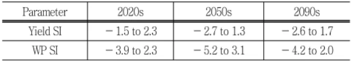
4. Uncertainty of Yield and WP

Table 6 shows the average (and range) standardized index (SI) of the simulated WP and yield. The standardized index (SI) captures the anomalies as a single numeric value; it shows the parameter deviation from the mean and is expressed by:

SI＝(x-x) / σ (5)

where x is the parameter value, x is the parameter mean and σ is the standard deviation.

If a normal distribution is assumed, index values greater than 1.5 denote significantly higher parameter values and those less than －1.5 denote significantly lower values. The condition is said to be near normal for SI values ranging from －0.99 to ＋0.99. At least two models in the A2 and A1B scenarios predict yields that are significantly different from the others while at least one model is significantly different in the 2050s and 2090s for the B1 scenario. The B1 scenario therefore has the least uncertainty. The WP is more uncertain than the yield. The high uncertainty is derived from the uncertainty from the evaporated quantity of water.

For each scenario at least three GCMs projected WP values that are significantly different from the others.

Table 6 Ranges of the standardized index (SI) of the simulated yield and WP

Parameter 2020s 2050s 2090s

Yield SI －1.5 to 2.3 －2.7 to 1.3 －2.6 to 1.7 WP SI －3.9 to 2.3 －5.2 to 3.1 －4.2 to 2.0

The method used here is a holistic system where it is difficult to trace uncertainty back to particular biases. The range of projected outcomes acts to integrate these dis- crepancies into a model-based uncertainty that can be thought of as a proxy of the actual uncertainty of yield due to climate change. The precision of impacts response surfaces regressed from crop model simulations is likely to depend on the crop, region, and degree to which yield changes are sensitive to particular climatic variables. In Zimbabwe, maize is grown under diverse conditions and it is likely that very few (if any) farms follow the exact specifications of the calibrated configuration. Whilst climate change will significantly shift the water balance, the ambient temperatures are predicted to remain within the optimum range. In irrigated agriculture, the maximum potential yields will increase as a result of the direct impact of the increased atmospheric CO2. How- ever, socio-economic and political factors which are beyond the scope of climate change complicate the relationship between crop yields and the climatic factors.

IV. CONCLUSIONS

The study presents a method to predict the impacts of climate change on the yield of maize and assess the associated uncertainty in three high maize production provinces of Zimbabwe. Evaporation was simulated to gradually increase over the future periods at a higher rate than the transpiration and had higher uncertainty. The maximum potential maize yields were simulated to increase by an average (and range) of 8 % (6-9 %), 14% (10-15 %) and 16 % (11-17 %) in the 2020s, 2050s and 2090s respectively. The WP was also projected to increase by an average (and range) of 7 % (4-13 %), 13 % (6-30 %) and 15 % (6-23 %) in the 2020s, 2050s and 2090s respectively. In Zimbabwe, maize is grown under diverse conditions and socio-economic and political factors which are beyond the scope of climate change complicate the relationship between crop yields and the climatic factors.

It is hoped that this study will encourage similar analyses for other crops and regions to determine what patterns exist in climate impacts uncertainty, and to develop ways of communicating uncertainty in the Zimbabwean context.

(9)

This research was supported by Basic Science Research Program through the National Research Foundation of Korea (NRF) funded by the Ministry of Education, Science and Technology (No. 2010-0007884) and by Kyungpook National University Research Fund, 2012.

REFERENCES

1. Cane, M. A., G. Eshel and R. W. Buckland, 1994.

Forecasting Zimbabwean maize yield using eastern equatorial Pacific sea surface temperature.

Nature

370:

204-205.

2. Chung, S.-O. and T. Nkomozepi, 2012. Uncertainty of paddy irrigation requirement estimated from climate change projections in the Geumho river basin, Korea.

Paddy and Water Environment

. published online DOI:

10.1007/s10333-011-0305-z.

3. Chung, S.-O., 2009. Climate change impacts on paddy irrigation requirement in the Nakdong river basin.

Journal of the KSAE

51(2): 35-41 (in Korean).

4. Chung, S.-O., 2010. Simulating evapotranspiration and yield responses of rice to climate change using FAO- AquaCrop.

Journal of the KSAE

52(3): 57-67 (in Korean).

5. Droogers, P. and R. G. Allen, 2002. Estimating reference evapotranspiration under inaccurate data conditions.

Irrigation and Drainage Systems

16: 33-45.

6. FAO (Food and Agriculture Organization), 2006.

Fertilizer use by crop in Zimbabwe.

ftp://ftp.fao.org/agl/agll/docs/

fertusezimbabwe.pdf accessed on 8 Jan, 2012.

7. Fildes, R. and N. Kourentzes, 2011. Validation and forecasting accuracy in models of climate change.

International Journal of Forecasting

27: 968-995.

8. Harrison, L., J. Michaelsen, C. Funk, and G. Husak, 2011.

Effects of temperature changes on maize production in Mozambique.

Climate Research

46: 211-222.

9. Holzkämper A., P. Calanca, and J. Fuhrer, 2012. Statistical crop models: predicting the effects of temperature and precipitation changes.

Climate Research

51:11-21.

10. Hong, E. M., J. Y. Choi, S. H. Lee, S. H. Yoo and M. S.

Kang, 2009. Estimation of paddy rice evapotranspiration considering climate change using LARS-WG.

Journal of the KSAE

51(3): 25-35 (in Korean).

11. Manatsa, D., I. W. Nyakudya, G. Mukwada, and H.

Matsikwa, 2011. Maize yield forecasting for Zimbabwe farming sectors using satellite rainfall estimates.

Natural Hazards

59: 447-463.

12. New, M., D. Lister, M. Hulme and I. Makin, 2002. A high resolution data set of surface climate over global land areas.

Climate Research

21: 1-25.

13. Nkomozepi, T. and S.-O. Chung, 2011a. Assessing the effects of climate change on irrigation water requirements for corn in Zimbabwe.

Journal of the KSAE

53(1): 47-55.

14. Nkomozepi, T. and S.-O. Chung, 2011b. Simulation of the effects of climate change on yield of maize in Zimbabwe.

Journal of the KSAE

53(3): 65-73.

15. Nkomozepi, T. and S.-O. Chung, 2012. Assessing the trends and uncertainty of maize net irrigation water requirement estimated from climate change projections for Zimbabwe.

Agricultural Water Management.

published online DOI:10.1016/j.agwat.2012.05.004.

16. Nyakudya, I. W. and L. Stroosnijder, 2011. Water management options based on rainfall analysis for rain fed maize (Zea mays L.) production in Rushinga district, Zimbabwe.

Agricultural Water Management

98: 1649- 1659.

17. Raes, D., A. Sithole, A. Makarau, and J. Milford, 2004.

Evaluation of first planting dates recommended by criteria currently used in Zimbabwe.

Agricultural and Forest Meteorology

125: 177-185.

18. Raes, D., P. Steduto, T. C. Hsiao, and E. Fereres, 2010.

AquaCrop reference manual

, AquaCrop version 3.1, FAO, Land and Water Division, Rome, Italy.

19. Ruane, A. C., L. D. Cecil, R. M. Horton, R. Gordon, R.

McCollum, D. Brown, B. Killough, R. Goldberg, A. P.

Creeley, and C. Rosenzweig, 2011. Climate change impact uncertainties for maize in Panama: Farm information, climate projections, and yield sensitivities.