Nelson AC, Moody M. 2003. Paying for Prosperity:
Impact Fees and Job Growth . Working paper.
Brookings Institution. Center on Urban and Metropolitan Policy.
Nicholas JC, Juergensmeyer JC. 1991. A Practitioner's Guide to Development Impact Fees .
Ord JK, Getis A. 1995. Local Spatial Autocorrelation Statistics: Distributional Issues and an Application.
Geographical Analysis . 27(4): 286-306.
Porter DR. 2012. Managing Growth in America's
Communities . Island Press.
Yinger J. 1998. The Incidence of Development Impact Fees and Special Assessments. National Tax Journal . 51: 23–41.
2017년 10월 5일 원고접수(Received) 2017년 11월 21일 1차심사(1st Reviewed) 2017년 12월 5일 2차심사(2nd Reviewed) 2017년 12월 8일 게재확정(Accepted)
초 록
최근 기반시설부담구역 지정의 객관성 확보를 위해 핫스팟(Hotspot) 분석기법과 같이 LISA에 기초한 공 간통계기법을 적용하려는 시도(Kim and Choei 2017)가 이루어진 바 있다. 그러나 Hotspot 방법의 경우 군 집여부를 판별하는 통계량 생산 이후에 이 정보를 바탕으로 구체적인 범역을 객관적으로 설정하기 위한 검증된 방법론을 추가 적용할 필요가 있으며, 본 연구는 이러한 맥락에서 유일 범역의 지정을 위한 AMOEBA 기법을 그 대안으로 채택하여 이전의 Hotspot 방식과 구역지정 결과를 비교검토해 보았다. 이를 위해 분석격자단위를 100m에서 400m까지 순차 증가시키는 시나리오 분석을 수행하고 단위면적당 개발 허가 건수 및 원형도의 두 가지 평가치로 비교평가해 보았다. 분석결과, 두 방식의 수치적 평가치는 유사 하였음에도, 적정 크기의 영역획정에서는 전자가, 기반시설설치 용이성에서는 후자가 다소 우월함을 보였 다. 특히 유사한 평가수치와는 달리 각 방식에 의한 지정구역의 40%는 서로 상이한 지역을 획정하고 있음 을 알 수 있는데, 이는 두 방식 간에 위치 적정성 판단기준에 유의미한 차이가 있음을 반증하는 것으로 보 이며, 따라서 이러한 구역지정 편차의 원인과 의미를 파악하기 위한 후속연구가 필요할 것으로 판단된다.
주요어 : 기반시설부담구역제도, 아메바 분석, 핫스팟 분석, 이행대, 제1단계구역
Analysis of Spatio-Temporal Patterns of Nighttime Light Brightness of Seoul Metropolitan Area
using VIIRS-DNB Data
*VIIRS-DNB 데이터를 이용한 수도권 야간 빛 강도의 시·공간 패턴 분석
Zhu, Lei
**∙ Cho, Daeheon
***∙ Lee, Soyoung
****주뢰
**∙ 조대헌
***∙ 이소영
****Abstract
Visible Infrared Imaging Radiometer Suite Day-Night Band (VIIRS-DNB) data provides a much higher capability for observing and quantifying nighttime light (NTL) brightness in comparison with Defense Meteorological Satellite-Operational Linescan System (DMSP-OLS) data. In South Korea, there is little research on the detection of NTL brightness change using VIIRS-DNB data.
This study analyzed the spatial distribution and change of NTL brightness between 2013 and 2016 using VIIRS-DNB data, and detected its spatial relation with possible influencing factors using regression models. The intra-year seasonality of NTL brightness in 2016 was also studied by analyzing the deviation and change clusters, as well as the influencing factors. Results are as follows: 1) The higher value of NTL brightness in 2013 and 2016 is concentrated in Seoul and its surrounding cities, which positively correlated with population density and residential areas, economic land use, and other factors; 2) There is a decreasing trend of NTL brightness from 2013 to 2016, which is obvious in Seoul, with the change of population density and area of industrial buildings as the main influencing factors; 3) Areas in Seoul, and some surrounding areas have high deviation of the intra-year NTL brightness, and 71% of the total areas have their highest NTL brightness in January, February, October, November and December; and 4) Change of NTL brightness between summer and winter demonstrated a significantly positive relation with snow cover area change, and a slightly and significantly negative relation with albedo change.
Keywords: VIIRS-DNB nighttime light, Spatio-temporal pattern, Spatial regression modelling, Seasonality, Spatial cluster analysis
* This research was supported by a grant (14NSIP-B080144-01) from National Land Space Information Research Program funded by Ministry of Land, Infrastructure and Transport of Korean government
** 서울대학교 지리교육과 박사수료 Department of Geography Education, Seoul National University (First author: [email protected]) *** 가톨릭관동대학교 지리교육과 조교수 Assistant Professor, Department of Geography Education, Catholic Kwandong
University (Corresponding author: [email protected])
**** 서울대학교 지리교육과 박사수료 Department of Geography Education, Seoul National University ([email protected])
1. Introduction
One of the vital alterations to the natural environment is the change of light brightness levels at night affected by increasing artificial light (Cinzano et al. 2001). Artificial light provides conveniences and advantages to our life, however, research shows that increased use of nighttime light (NTL) has become the main elements of the environmental pollution (Han et al. 2014).
According to International Dark-Sky Association (IDA), light pollution is the inappropriate or excessive use of artificial light, including skyglow, glare, light trespass and clutter (http://www.
darksky.org/light-pollution/). Research on the light pollution in global scale shows that 19% of the total land surface has a brightness above the light pollution threshold (Cinzano et al. 2001).
Many studies have been performed on the adverse effect of light pollution on flora and fauna (Aubrecht et al. 2009; Horváth et al. 2009; Inger et al. 2014; Nordt and Klenke 2013), as well as human health such as inducing breast or prostate cancer(Cinzano et al. 2001; Falchi et al. 2011;
Kloog et al. 2008; Kloog et al. 2009; Kloog et al.
2010).
Quantifying the brightness of artificial light at night has attached more and more attention as a first step of NTL researches such as light pollution estimation (Bennie et al. 2014). Therefore, many studies have been conducted on the measurement of NTL brightness, among which, site survey using measurement devices is widely adopted in local scale. For example, in order to identify the actual
situation of artificial light, Lee et al. (2013) introduced a method to create 3D light map through site survey using GPS. However, this method is not suitable for evaluating NTL brightness in city or regional scale, instead, nighttime remote sensing images become frequently adopted.
In studies on NTL, the nighttime data collected by the U.S. Air Force Defense Meteorological Satellite - Operational Linescan System (DMSP- OLS) sensors have been mainly used until 2000s, as shown in details by Huang et al. (2014). Since 2011, DNB (Day and Night Band) of VIIRS (Visible Infrared Imaging Radiometer Suite) data on SNPP (Soumi National Polar-orbiting Partnership) satellite have been much more widely utilized due to its superiority to DMSP-OLS data. VIIRS-DNB data is evaluated to be more enhanced with reduced spatial saturation and over-glow, superior calibration, better radiometric and spatial resolution (Lee et al. 2006).
Due to the merits of NTL data, it has been widely applied in various fields for different aims, and the studies can be divided into several types as follows:
First, many analysis on spatial pattern and spatio-temporal change of NTL brightness have been conducted as a method to quantify NTL pollution. For example, Bennie et al. (2014) detected NTL brightness decreases and increases across Europe from 1995 to 2010 with calibrated DMSP-OLS data to identify the trends of light pollution. Xiang and Tan (2017) used calibrated DMSP-OLS data to study light pollution change in protected areas in China from 1992 to 2011,
showing that areas of light pollution increased due to human activities and intrinsic factors.
Second, NTL data is widely used for detecting geographical characteristics of human activities, like urban boundary or urban expansion extraction
(Liu et al. 2012; Shi et al. 2014; Zhu et al. 2016), population modelling (Sutton et al. 2001; Yoo et al.
2011), and electricity consumption estimation (Chand et al. 2009; Shi et al. 2014).
Third, analyses on relation between NTL data and subsequent ecological problems (Aubrecht et al. 2009), and human health problems (Kloog et al.
2008; Kloog et al. 2009; Kloog et al. 2010) are also widely performed.
Forth, analysis on the influencing factors of spatial pattern and spatio-temporal change of NTL brightness is getting attention recently. For example, Levin and Zhang (2017) analyzed factors explaining VIIRS NTL brightness levels from densely populated areas, and results showed both socio-economic variables like GDP per capita, MODIS derived percent urban area, density of road network, and physical variables like NDVI values, snow cover area, and latitude all contributed to NTL brightness. Levin (2017) observed the seasonal changes of NTL in central and northern America using VIIRS-DNB data, and analyzed the relation between NTL brightness change and seasonal change of albedo, especially changes related to variety of NDVI and snow cover.
In South Korea (hereafter, Korea), there are few studies on NTL brightness analysis in regional and national scales. In addition, the analysis on influencing factors of spatial pattern and spatio- temporal change of NTL brightness is rarely seen.
Therefore, we pay attention to the spatial pattern and change of NTL brightness and its influencing factors in this study. Specially, according to the previous research which indicated seasonal changes in landscape patterns may be greater (Lambin 1996), and it is also proposed that for light pollution analysis, the seasonal increase of NTL brightness should be taken into account to understand the impacts of artificial light on ecological rhythms and human health (Levin 2017), we analyzed both inter-year change, and the seasonal (intra-year) change of NTL brightness.
This study aims to analyze spatio-temporal pattern and the possible influencing factors of NTL brightness in 2013 and 2016 in Seoul metropolitan area. For this purpose, first, we analyzed the spatial pattern and change of NTL brightness in 2013 and 2016; second, we identified the influencing factors of the spatial pattern and change; third, we studied the seasonality of NTL brightness and its influencing factors. The study proceeds as follows. Section 2 introduces the study area, data and methods used in this study. Section 3 presents the analysis results. Section 4 depicts discussion of the analysis results and conclusions.
2. Data and Methods 2.1. Study area and spatial unit
This study mainly focuses on the Seoul
metropolitan area of Korea, including Seoul,
Incheon and Gyeonggi-do. By analyzing NTL
image, we found that cluster areas of cells with
(a) (b)
Figure 1. NTL in 2013 (a) and 2016 (b)
digital number (DN) above mean were mainly less than Eup-Myeon-Dong (hereafter, EMD) administrative unit, therefore, we estimated that analysis in Si-Gun-Gu unit would excessively smooth the original data. So spatial unit of this study was defined as EMD unit considering the locally concentrated tendency of distribution and change of NTL brightness. We unified the spatial unit into EMD unit of 2013 while merging and modifying some areas. Due to the lack of data resources and the spatial separation, some areas are deleted or modified, resulting in a study area with 1106 units.
2.2. Data resources
The main data used in this study are VIIRS-DNB data, and data of influencing factors
of spatio-temporal pattern of NTL brightness, as shown in Table 1.
2.2.1. Data of NTL brightness: VIIRS- DNB
We used monthly VIIRS-DNB cloud-free composites Tile 1 (75N060E, which covers the total area of Korea) derived from National Centers for Environmental Information (NOAA, https://
ngdc.noaa.gov/eog/viirs/download_dnb_composit es.html). The monthly composites are produced by averaging daily nighttime data derived, and before averaging, the data are all atmospherically corrected to exclude the impact of stray light, lightning, lunar illumination, and cloud cover by Earth Observation Group (EOG) at NOAA/NGDC (Hillger et al. 2013). Twenty-four average radiance composite monthly images (from January
to December in 2013, and 2016 respectively) were downloaded. The original spatial resolution of VIIRS-DNB data is 15 arc sec (about 500m at the equator), with a unit in nanoWatts/cm
2/sr. In this study, the data were resampled into a spatial resolution of 500m using nearest neighbor method, as shown in Figure 1, in order to match the cell size of Moderate Resolution Imaging Spectroradiometer (MODIS) data for seasonality analysis, and then conducted zonal statistics by averaging DN value into END unit for 2013 and 2016 respectively. For that there are missing values in majority of the study area in both June and July, the data of these two months were excluded, so the other 10 months in both 2013 and 2016 were used.
2.2.2. Data of possible influencing factors
1) Influencing factors of spatial pattern and change of NTL brightness in 2013 and 2016
In order to detect possible influencing factors of NTL brightness distribution, anthropological factors, such as population density (Elvidge et al.
1997), road area density (Levin and Zhang 2017), and the building area proportions with various building types (residential, commercial, industrial, office, public, agricultural and other types) were selected. The detail ancillary data and their sources are shown in Table 1.
2) Influencing factors of NTL brightness seasonal change in 2016
We used seasonal variables, snow cover area, NDVI and albedo, to evaluate the seasonality of NTL brightness.
Monthly snow cover data were downloaded from MODIS/Terra Snow Cover 8-Day L3 Global 500m Grid, Version 6 (MOD10A2) collection. This dataset is produced by compositing 8 days of the daily tile products with area being classified into snow covered area if the snow is detected on any day on the daily tile product. Therefore this composite represents the maximum snow cover during the 8-day period (Hall and Riggs 2007). Monthly snow cover composites were generated by averaging the initial 8-day composites. Also, snow cover data were examined by referring to the historical weather data to exclude errors. The monthly composited snow cover data were also conducted zonal statistics by averaging into the study units.
MODIS/Terra Vegetation Indices 16-Day L3 Global 500m SIN Grid, Version 006 (MOD13A1) collection were downloaded. NDVI of this dataset were used to represent the vegetation cover. Like snow cover data, NDVI data were also conducted into monthly composites and averaged into study areas.
For the albedo data, the Albedo 16-Day L3 Global 500m (MCD43A3) collection were downloaded. In this study, White-Sky Albedo in the visible spectral range was used. Also, the albedo data were aggregated into monthly composites, and averaged into study areas.
In order to study the seasonality of NTL in 2016,
all of the MODIS data were derived from January
1st to December 31st of 2016. Furthermore, in
order to validate the no-data value in initial
MODIS images, interpolation was conducted
(Levin 2017).
Data Variable Source
NTL brightness data VIIRS-DNB
National Centers for Environmental Information
https://ngdc.noaa.gov/eog/viirs/index.html
MODIS data
MOD10A2 snow cover area Land Process Distributed Active Archive Center
https://lpdaac.usgs.gov/
MOD13A1 NDVI MCD43A3 albedo
Population data Population density KOSIS
http://kosis.kr/index/index.jsp
Building use type data
Residential building area
Database of Road Name Address System
http://www.juso.go.kr/addrlink/addrlinkJuso DBUse.do?menu=main
Commercial building area Industrial building area
Office building area Public building area Agricultural building area
Other building area Road area data Road density Table 1. Data and sources
2.3. Methods
In order to figure out the aspatial and spatio- temporal characteristics of NTL brightness distribution and change, we presented the basic descriptive statistics, and conducted spatial cluster analysis.
For influencing factor analysis of the spatio- temporal pattern of NTL brightness, principal component analysis (PCA) and regression modelling were applied.
2.3.1. Spatial cluster analysis
In order to identify local cluster distribution of NTL brightness change, spatial statistical analysis was performed. Local indicator
and
have good performance on cluster detection (Getis et al.
2010).
The statistics of
is defined as follows:
Where
where is the number of spatial units indexed by and , is the variable of interest, is the mean of , and
is an element of a spatial weight matrix.
is 1 if shares a boundary with
, 0 otherwise. And hot spots indicate a high values (above mean) surrounded by high values, while cold spots indicate low values (lower than mean) surrounded by low values.
(1)
2.3.2. Regression modelling
Regression modelling was applied to analyze the relation between distribution and change of NTL brightness and the possible influencing factors.
Before modelling, PCA was performed to reduce multicollinearity of influencing factors. And factors with eigenvalues above 1 were selected as independent variables of the subsequent regression analysis.
If the dependent variables themselves have spatial autocorrelation, the residuals can be autocorrelated with each other. Autocorrelated residuals are against the independence assumption for errors in the standard regression model. If the residuals are spatially autocorrelated, the error items are not independent, and so the regression parameter estimates are no longer the best linear unbiased estimator (BLUE) (Voss et al. 2006).
In order to exclude the spatial autocorrelation of residuals, the spatial error model (SEM) was used, which is specified (matrix notation) as follows:
where is a × vector representing the dependent variable, is a × matrix representing the independent variables, is a × vector of regression parameters to be estimated, is a × vector of error terms presumed to have a covariance structure as given in the second equation, is a spatial autoregressive coefficient, and is a × spatial weight matrix defining neighborhood structure, and as the spatial weight matrix of
, the weight equals to 1 if and share a boundary, otherwise 0.
Even though we focused on SEM, ordinal least squares (OLS) model was also applied when analyzing the influencing factors of NTL brightness spatial distribution in 2013 as a reference to SEM.
All of these calculations were performed in GeoDa and spatial analysis tools that were developed by Opensource GIS Project of National Land Space Information Program, the name of which is “Development of Opensource Geospatial Software” (Korea Agency for Infrastructure Technology Advancement 2017).
3. Results
3.1. Spatial distribution and change of NTL brightness
3.1.1. Aspatial characteristics of NTL
brightness in 2013 and 2016
First, we presented the aspatial characteristics
of NTL brightness in 2013 and 2016 by dividing
the total NTL brightness into 5 levels and
analyzing the area proportion and the brightness
proportion of each level. Results are shown in
Table 2. We can see that in 2013, a majority of
areas (about 84%) have NTL brightness at 10~100
(unit in nanoWatts/cm
2/sr, hereafter), and there
are only 13 among 1106 areas have brightness
above 100, while 157 areas have low brightness
under 10. From area proportion and brightness
proportion, we can see the concentricity of the
NTL brightness, because 71% of the total area
assumes 1% of the total NTL brightness, while the
other 99% of NTL concentrates in only 29% of the
(2)
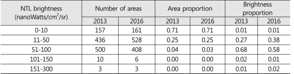
total area. As with 2013, NTL also shows a great concentration in 2016. There are 936 areas among 1106 (about 85%) areas that have NTL brightness of 10~100, while there are only 9 areas that have NTL brightness above 100. Although the area with brightness under 10 assumes 71% of the total area, it covers only 2% of the total NTL brightness, while the other 98% of the total brightness is concentrated in only 29% of the total area. We can see that although the brightness proportion of the highest level increased, there is a decreasing trend of NTL brightness from 2013 to 2016. This observation will be analyzed in detail later.
3.1.2. Spatial distribution and change of NTL brightness
Applying the above classification on spatial dimension, we can see from Figure 2 that there is a high concentration of NTL brightness, mainly distributed around Seoul in both 2013 and 2016. In 2013, areas of highest brightness are located in Jung-gu and Jongno-gu in Seoul, which have brightness above 150, and the periphery areas of Gyeonggi-do and Ganghwa-gun of Incheon have very low NTL brightness intensity, which is under
10. In 2016, it also shows the same high concentration in the central area of Seoul, some areas in Incheon and some surrounding cities of Seoul such as Suwon-si, Seongnam-si, Anyang-si in Geyonggi-do. In comparison with NTL brightness distribution of 2013, the main characteristic of 2016 is the increase of the lower brightness areas (brightness under 100) as well as the decrease of the higher brightness areas (brightness above 100), especially in some areas of Dongjak-gu, Yeongdeungpo-gu, Seongdong-gu of Seoul.
As mentioned, there is a decreasing trend of NTL brightness from 2013 to 2016. Table 3 shows the descriptive statistics of the total 1106 units and mean value of Seoul, Incheon, and Gyeonggi- do. We can see that the total brightness and the mean value are decreasing. On the other side, the maximum in 2016 is a little higher than that of 2013, while the minimum is lower. The mean values of Seoul, Incheon, and Gyeonggi-do in 2013 and 2016 in Table 3 show the highest value concentration in Seoul and a lower mean NTL brightness of the three areas in 2016 than that in 2013.
NTL brightness (nanoWatts/cm2/sr)
Number of areas Area proportion Brightness proportion
2013 2016 2013 2016 2013 2016
0-10 157 161 0.71 0.71 0.01 0.01
11-50 436 528 0.25 0.25 0.27 0.38
51-100 500 408 0.04 0.03 0.68 0.58
101-150 10 6 0.00 0.00 0.02 0.01
151-300 3 3 0.00 0.00 0.01 0.02
Table 2. Distribution of NTL brightness in 2013 and 2016
* Number of areas is the number of EMD unit; Area proportion and brightness proportion is calculated by dividing the sum of area and NTL brightness in every class by the total area and total NTL brightness.
(a) (b)
Figure 2. NTL brightness distribution of 2013 (a) and 2016 (b)
(a) (b)
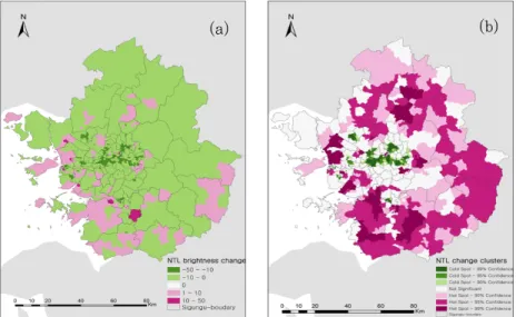
Figure 3. Spatial distribution of NTL brightness change (a) and clusters of change (b)
Table 3. NTL change from 2013 to 2016 (nanoWatts/cm2/sr)
Year Descriptive statistics for the entire area Seoul (Mean)
Incheon (Mean)
Gyeonggi-do (Mean)
Sum Mean STD Maximum Minimum
2013 49371.66 44.64 27.68 265.86 0.46 48.73 18.19 8.07
2016 44449.39 40.19 25.42 271.99 0.35 42.78 17.59 7.57
total area. As with 2013, NTL also shows a great concentration in 2016. There are 936 areas among 1106 (about 85%) areas that have NTL brightness of 10~100, while there are only 9 areas that have NTL brightness above 100. Although the area with brightness under 10 assumes 71% of the total area, it covers only 2% of the total NTL brightness, while the other 98% of the total brightness is concentrated in only 29% of the total area. We can see that although the brightness proportion of the highest level increased, there is a decreasing trend of NTL brightness from 2013 to 2016. This observation will be analyzed in detail later.
3.1.2. Spatial distribution and change of NTL brightness
Applying the above classification on spatial dimension, we can see from Figure 2 that there is a high concentration of NTL brightness, mainly distributed around Seoul in both 2013 and 2016. In 2013, areas of highest brightness are located in Jung-gu and Jongno-gu in Seoul, which have brightness above 150, and the periphery areas of Gyeonggi-do and Ganghwa-gun of Incheon have very low NTL brightness intensity, which is under
10. In 2016, it also shows the same high concentration in the central area of Seoul, some areas in Incheon and some surrounding cities of Seoul such as Suwon-si, Seongnam-si, Anyang-si in Geyonggi-do. In comparison with NTL brightness distribution of 2013, the main characteristic of 2016 is the increase of the lower brightness areas (brightness under 100) as well as the decrease of the higher brightness areas (brightness above 100), especially in some areas of Dongjak-gu, Yeongdeungpo-gu, Seongdong-gu of Seoul.
As mentioned, there is a decreasing trend of NTL brightness from 2013 to 2016. Table 3 shows the descriptive statistics of the total 1106 units and mean value of Seoul, Incheon, and Gyeonggi- do. We can see that the total brightness and the mean value are decreasing. On the other side, the maximum in 2016 is a little higher than that of 2013, while the minimum is lower. The mean values of Seoul, Incheon, and Gyeonggi-do in 2013 and 2016 in Table 3 show the highest value concentration in Seoul and a lower mean NTL brightness of the three areas in 2016 than that in 2013.
NTL brightness (nanoWatts/cm2/sr)
Number of areas Area proportion Brightness proportion
2013 2016 2013 2016 2013 2016
0-10 157 161 0.71 0.71 0.01 0.01
11-50 436 528 0.25 0.25 0.27 0.38
51-100 500 408 0.04 0.03 0.68 0.58
101-150 10 6 0.00 0.00 0.02 0.01
151-300 3 3 0.00 0.00 0.01 0.02
Table 2. Distribution of NTL brightness in 2013 and 2016
* Number of areas is the number of EMD unit; Area proportion and brightness proportion is calculated by dividing the sum of area and NTL brightness in every class by the total area and total NTL brightness.
(a) (b)
Figure 2. NTL brightness distribution of 2013 (a) and 2016 (b)
(a) (b)
Figure 3. Spatial distribution of NTL brightness change (a) and clusters of change (b)
Table 3. NTL change from 2013 to 2016 (nanoWatts/cm2/sr)
Year Descriptive statistics for the entire area Seoul (Mean)
Incheon (Mean)
Gyeonggi-do (Mean)
Sum Mean STD Maximum Minimum
2013 49371.66 44.64 27.68 265.86 0.46 48.73 18.19 8.07
2016 44449.39 40.19 25.42 271.99 0.35 42.78 17.59 7.57
(b) (a)
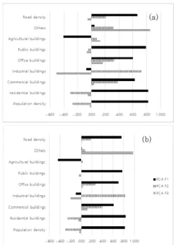
Figure 4. Factor loadings of variables in PCA of 2013 (a) and 2016 (b)
In order to investigate the spatial and temporal change of NTL brightness from 2013 to 2016, the spatial distribution of NTL brightness change and the change clusters were studied, as shown in Figure 3. We can see that a majority of areas have lower NTL brightness in 2016 than in 2013. This situation is more obvious in some areas of Seoul.
On the other hand, the periphery areas of Gyeonggi-do, such as Hwaseong-si, Yeoju-si, Pyeongtaek-si, and Jung-gu, Seo-gu of Incheon have higher NTL brightness in 2016. By calculation, only 19.2% of the total study areas have increasing NTL brightness, while other 80.8% show a decrease of NTL brightness. From the cluster detection analysis by calculating
values, we can see that cold spots (clusters of areas with change value lower than the average change value) are mainly distributed in Seoul, and the hot spots (clusters of areas with change value higher than the average change value) are mainly in the periphery areas of Gyeonggi-do.
3.2. Modelling of the spatial distribution and change pattern of NTL brightness
3.2.1. Modelling of the spatial distribution of NTL brightness in 2013 and 2016 Regression models (OLS and SEM) have been applied to evaluate the relation between NTL brightness and the possible influencing factors. In order to reduce multicollinearity, PCA was performed and the first three factors with eigenvalues above 1 are selected (37.1%, 12.1%, and 11.4% for 2013, and 40.2%, 12.3% and 11.3%
for 2016). With high similarity in 2013 and 2016,
we can see that the F1 is positively correlated with the population density and residential areas (population density, road density, and commercial and residential buildings), and F2 is positively related to economic land use, such as areas with high road density, and high proportion of commercial and industrial areas. The third factor is highly related to other types, as shown in Figure 4.
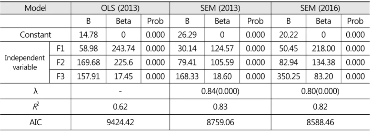
The results of OLS and SEM are as Table 4. We can see that in 2013, all of the three factors are positively related to NTL brightness and the goodness of fit increased obviously when the spatial autocorrelation of errors was considered.
And from the standardized coefficient, we can see that the first factor, population density and residential areas, has the highest influence on NTL brightness distribution, while the economic land
Model OLS (2013) SEM (2013) SEM (2016)
B Beta Prob B Beta Prob B Beta Prob
Constant 14.78 0 0.000 26.29 0 0.000 20.22 0 0.000
Independent variable
F1 58.98 243.74 0.000 30.14 124.57 0.000 50.45 218.00 0.000 F2 169.68 225.6 0.000 79.41 105.59 0.000 82.94 134.38 0.000 F3 157.91 17.45 0.000 168.33 18.60 0.000 350.25 83.20 0.000
λ - 0.84(0.000) 0.80(0.000)
R
2 0.62 0.83 0.82AIC 9424.42 8759.06 8588.46
* B is the unstandardized coefficient, Beta is the standardized coefficient, Prob is the probability, the same below.
Table 4. Results of NTL brightness distribution modelling
use also shows a little lower but relatively high influence.
SEM has an increased goodness of fit, which means a better explanation of the independent variable. Only SEM was performed on the dataset of 2016 in order to detect the dependent relationship between NTL brightness and the factors of PCA. The results are as Table 4. We can see that the factors, population density and residential areas, economic land use and the other factors, all have a positive relationship with the distribution of NTL brightness. The standard coefficient of F1, F2 and F3 are 218.00, 134.38 and 83.20 respectively, showing that the factor about population density or residential areas influences the NTL brightness distribution the most in 2016, and the economic land use also shows a relatively high influence.
3.2.2. Modelling of the change pattern of NTL brightness from 2013 to 2016 Same factors are used to identify possible
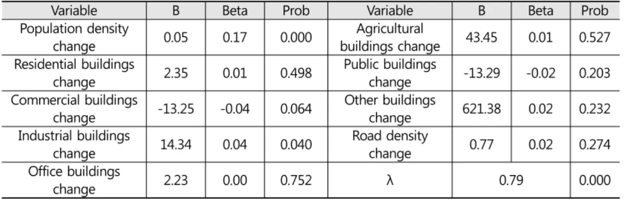
influencing factors of NTL brightness change. The change of population density, road density and the area change of different types of buildings were assumed as independent variables, with change of NTL brightness as dependent variable. Due to the reason that some buildings and road density tend to change slightly, PCA was not performed here. The VIF values of factors are less than 2, showing little possibility of multicollinearity. Thus the variables were directly applied into regression model. In addition, SEM was been performed, which resulted in an
of 0.58. The results are shown in Table 5.
For the results, except for commercial and
public buildings, other variables all positively
related to NTL brightness change. According to
the standardized coefficients, we can see that the
main influencing factor for NTL brightness
change is population density change and
industrial buildings change. Although it has a little
higher p-value, commercial buildings can also be
seen negatively contributed to the change of NTL
(b) (a)
Figure 4. Factor loadings of variables in PCA of 2013 (a) and 2016 (b)
In order to investigate the spatial and temporal change of NTL brightness from 2013 to 2016, the spatial distribution of NTL brightness change and the change clusters were studied, as shown in Figure 3. We can see that a majority of areas have lower NTL brightness in 2016 than in 2013. This situation is more obvious in some areas of Seoul.
On the other hand, the periphery areas of Gyeonggi-do, such as Hwaseong-si, Yeoju-si, Pyeongtaek-si, and Jung-gu, Seo-gu of Incheon have higher NTL brightness in 2016. By calculation, only 19.2% of the total study areas have increasing NTL brightness, while other 80.8% show a decrease of NTL brightness. From the cluster detection analysis by calculating
values, we can see that cold spots (clusters of areas with change value lower than the average change value) are mainly distributed in Seoul, and the hot spots (clusters of areas with change value higher than the average change value) are mainly in the periphery areas of Gyeonggi-do.
3.2. Modelling of the spatial distribution and change pattern of NTL brightness
3.2.1. Modelling of the spatial distribution of NTL brightness in 2013 and 2016 Regression models (OLS and SEM) have been applied to evaluate the relation between NTL brightness and the possible influencing factors. In order to reduce multicollinearity, PCA was performed and the first three factors with eigenvalues above 1 are selected (37.1%, 12.1%, and 11.4% for 2013, and 40.2%, 12.3% and 11.3%
for 2016). With high similarity in 2013 and 2016,
we can see that the F1 is positively correlated with the population density and residential areas (population density, road density, and commercial and residential buildings), and F2 is positively related to economic land use, such as areas with high road density, and high proportion of commercial and industrial areas. The third factor is highly related to other types, as shown in Figure 4.
The results of OLS and SEM are as Table 4. We can see that in 2013, all of the three factors are positively related to NTL brightness and the goodness of fit increased obviously when the spatial autocorrelation of errors was considered.
And from the standardized coefficient, we can see that the first factor, population density and residential areas, has the highest influence on NTL brightness distribution, while the economic land
Model OLS (2013) SEM (2013) SEM (2016)
B Beta Prob B Beta Prob B Beta Prob
Constant 14.78 0 0.000 26.29 0 0.000 20.22 0 0.000
Independent variable
F1 58.98 243.74 0.000 30.14 124.57 0.000 50.45 218.00 0.000 F2 169.68 225.6 0.000 79.41 105.59 0.000 82.94 134.38 0.000 F3 157.91 17.45 0.000 168.33 18.60 0.000 350.25 83.20 0.000
λ - 0.84(0.000) 0.80(0.000)
R
2 0.62 0.83 0.82AIC 9424.42 8759.06 8588.46
* B is the unstandardized coefficient, Beta is the standardized coefficient, Prob is the probability, the same below.
Table 4. Results of NTL brightness distribution modelling
use also shows a little lower but relatively high influence.
SEM has an increased goodness of fit, which means a better explanation of the independent variable. Only SEM was performed on the dataset of 2016 in order to detect the dependent relationship between NTL brightness and the factors of PCA. The results are as Table 4. We can see that the factors, population density and residential areas, economic land use and the other factors, all have a positive relationship with the distribution of NTL brightness. The standard coefficient of F1, F2 and F3 are 218.00, 134.38 and 83.20 respectively, showing that the factor about population density or residential areas influences the NTL brightness distribution the most in 2016, and the economic land use also shows a relatively high influence.
3.2.2. Modelling of the change pattern of NTL brightness from 2013 to 2016 Same factors are used to identify possible
influencing factors of NTL brightness change. The change of population density, road density and the area change of different types of buildings were assumed as independent variables, with change of NTL brightness as dependent variable. Due to the reason that some buildings and road density tend to change slightly, PCA was not performed here.
The VIF values of factors are less than 2, showing little possibility of multicollinearity. Thus the variables were directly applied into regression model. In addition, SEM was been performed, which resulted in an
of 0.58. The results are shown in Table 5.
For the results, except for commercial and
public buildings, other variables all positively
related to NTL brightness change. According to
the standardized coefficients, we can see that the
main influencing factor for NTL brightness
change is population density change and
industrial buildings change. Although it has a little
higher p-value, commercial buildings can also be
seen negatively contributed to the change of NTL
Variable B Beta Prob Variable B Beta Prob Population density
change 0.05 0.17 0.000 Agricultural
buildings change 43.45 0.01 0.527 Residential buildings
change 2.35 0.01 0.498 Public buildings
change -13.29 -0.02 0.203
Commercial buildings
change -13.25 -0.04 0.064 Other buildings
change 621.38 0.02 0.232
Industrial buildings
change 14.34 0.04 0.040 Road density
change 0.77 0.02 0.274
Office buildings
change 2.23 0.00 0.752 λ 0.79 0.000
Table 5. Result of NTL brightness change modelling
brightness to some degree. The model indicates that the decrease of population density and the decrease of area of industrial buildings, significantly led to the decrease of NTL brightness.
3.3. The seasonality of nighttime light brightness and possible influencing factors
Many studies have been conducted using monthly average composite of VIIRS-DNB data, besides inter-year change, intra-year change of NTL brightness is getting more and more attention on various research themes. For example, Li et al.
(2015) detected the ISIS offensive against Iraq in 2014 using the monthly VIIRS-DNB NTL data, concluding that there is a major loss of city lighting in the Northern Iraq due to the conflict and a subsequent inaccessibility to electricity supply. Jaturapitpornchai et al. (2015) used the monthly VIIRS data of July, August and September to extract the urban area in Bangkok, Thailand.
Studies have shown that there is seasonality of VIIRS-DNB NTL brightness, with snow cover and
NDVI as possible affecting factors (Cinzano et al.
2000; Elvidge et al. 2001; Levin 2017). This section described the seasonality of the NTL brightness in EMD unit of Seoul metropolitan area in 2016 (from January 2016 to December 2106, excluding June and July), and investigated whether the factors such as NDVI, snow cover and albedo had any influence on NTL seasonality.
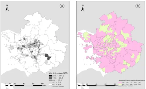
3.3.1. The seasonality of nighttime light First, in order to figure out the general characteristics of NTL brightness of each month, mean, STD, maximum and minimum of the total EMD units in every month were calculated, as shown in Table 6. It shows that the highest and lowest value of mean, STD, and maximum value are all distributed in October and May respectively, showing a high brightness and a more discrete distribution in October, and a low brightness and a concentrated distribution in May. The highest minimum values are in January and December, while the lowest minimum value are distributed in May and November. The differences of monthly NTL brightness can be seen more clearly in Figure 5 (with data in 2013 as a reference). We can see
Table 6. Descriptive statistics of monthly NTL brightness in 2016 (nanoWatts/cm2/sr)
Jan. Feb. Mar. Apr. May. Aug. Sep. Oct. Nov. Dec. Range
Mean 41.85 41.49 39.46 37.90 33.77* 40.99 34.59 46.00** 41.61 44.24 12.23 STD 25.61 25.71 27.15 23.59 19.74* 25.92 21.57 33.50** 27.32 30.00 13.76 Max. 305.35 218.54 353.43 260.63 169.10* 210.45 183.61 517.59** 324.95 445.62 348.49
Min. 0.42** 0.39 0.36 0.33 0.40 0.28 0.25* 0.39 0.25* 0.42** 0.17
* Lowest value. ** Highest value. Range is Max.-Min.
Figure 5. Average NTL brightness (nanoWatts/cm2/sr) of the entire units in every month
(a) (b)
Figure 6. Distribution of monthly NTL brightness STD (a) and Distribution of annual maximum (b)
Variable B Beta Prob Variable B Beta Prob Population density
change 0.05 0.17 0.000 Agricultural
buildings change 43.45 0.01 0.527 Residential buildings
change 2.35 0.01 0.498 Public buildings
change -13.29 -0.02 0.203
Commercial buildings
change -13.25 -0.04 0.064 Other buildings
change 621.38 0.02 0.232
Industrial buildings
change 14.34 0.04 0.040 Road density
change 0.77 0.02 0.274
Office buildings
change 2.23 0.00 0.752 λ 0.79 0.000
Table 5. Result of NTL brightness change modelling
brightness to some degree. The model indicates that the decrease of population density and the decrease of area of industrial buildings, significantly led to the decrease of NTL brightness.
3.3. The seasonality of nighttime light brightness and possible influencing factors
Many studies have been conducted using monthly average composite of VIIRS-DNB data, besides inter-year change, intra-year change of NTL brightness is getting more and more attention on various research themes. For example, Li et al.
(2015) detected the ISIS offensive against Iraq in 2014 using the monthly VIIRS-DNB NTL data, concluding that there is a major loss of city lighting in the Northern Iraq due to the conflict and a subsequent inaccessibility to electricity supply. Jaturapitpornchai et al. (2015) used the monthly VIIRS data of July, August and September to extract the urban area in Bangkok, Thailand.
Studies have shown that there is seasonality of VIIRS-DNB NTL brightness, with snow cover and
NDVI as possible affecting factors (Cinzano et al.
2000; Elvidge et al. 2001; Levin 2017). This section described the seasonality of the NTL brightness in EMD unit of Seoul metropolitan area in 2016 (from January 2016 to December 2106, excluding June and July), and investigated whether the factors such as NDVI, snow cover and albedo had any influence on NTL seasonality.
3.3.1. The seasonality of nighttime light First, in order to figure out the general characteristics of NTL brightness of each month, mean, STD, maximum and minimum of the total EMD units in every month were calculated, as shown in Table 6. It shows that the highest and lowest value of mean, STD, and maximum value are all distributed in October and May respectively, showing a high brightness and a more discrete distribution in October, and a low brightness and a concentrated distribution in May. The highest minimum values are in January and December, while the lowest minimum value are distributed in May and November. The differences of monthly NTL brightness can be seen more clearly in Figure 5 (with data in 2013 as a reference). We can see
Table 6. Descriptive statistics of monthly NTL brightness in 2016 (nanoWatts/cm2/sr)
Jan. Feb. Mar. Apr. May. Aug. Sep. Oct. Nov. Dec. Range
Mean 41.85 41.49 39.46 37.90 33.77* 40.99 34.59 46.00** 41.61 44.24 12.23 STD 25.61 25.71 27.15 23.59 19.74* 25.92 21.57 33.50** 27.32 30.00 13.76 Max. 305.35 218.54 353.43 260.63 169.10* 210.45 183.61 517.59** 324.95 445.62 348.49
Min. 0.42** 0.39 0.36 0.33 0.40 0.28 0.25* 0.39 0.25* 0.42** 0.17
* Lowest value. ** Highest value. Range is Max.-Min.
Figure 5. Average NTL brightness (nanoWatts/cm2/sr) of the entire units in every month
(a) (b)
Figure 6. Distribution of monthly NTL brightness STD (a) and Distribution of annual maximum (b)