http://dx.doi.org/10.7848/ksgpc.2015.33.3.211
Automatic Cross-calibration of Multispectral Imagery with Airborne Hyperspectral Imagery Using Spectral Mixture Analysis
Kim, Yeji
1)ㆍChoi, Jaewan
2)ㆍChang, Anjin
3)ㆍKim, Yongil
4)Abstract
The analysis of remote sensing data depends on sensor specifications that provide accurate and consistent measurements. However, it is not easy to establish confidence and consistency in data that are analyzed by different sensors using various radiometric scales. For this reason, the cross-calibration method is used to calibrate remote sensing data with reference image data. In this study, we used an airborne hyperspectral image in order to calibrate a multispectral image. We presented an automatic cross-calibration method to calibrate a multispectral image using hyperspectral data and spectral mixture analysis. The spectral characteristics of the multispectral image were adjusted by linear regression analysis. Optimal endmember sets between two images were estimated by spectral mixture analysis for the linear regression analysis, and bands of hyperspectral image were aggregated based on the spectral response function of the two images. The results were evaluated by comparing the Root Mean Square Error (RMSE), the Spectral Angle Mapper (SAM), and average percentage differences. The results of this study showed that the proposed method corrected the spectral information in the multispectral data by using hyperspectral data, and its performance was similar to the manual cross-calibration.
The proposed method demonstrated the possibility of automatic cross-calibration based on spectral mixture analysis.
Keywords : Cross-calibration, Spectral Mixture Analysis, Spectral Unmixing, Hyperspectral Image, Multispectral Image
Original article
Received 2015. 06. 11, Revised 2015. 06. 19, Accepted 2015. 06. 29
1) Member, Department of Civil and Environmental Engineering, Seoul National University (Email: [email protected]) 2) Member, School of Civil Engineering, Chungbuk National University (Email: [email protected]) 3) Member, Civil Engineering, Texas A&M University-Corpus Christi (Email: [email protected])
4) Corresponding Author, Member, Department of Civil and Environmental Engineering, Seoul National University (E-mail: [email protected])
This is an Open Access article distributed under the terms of the Creative Commons Attribution Non-Commercial License (http://
1. Introduction
As the number of Earth observation satellites has increased, an increasing amount of remote sensing data has been extended to applications of remote sensing in different fields of study. Remote sensing data acquired from multiple sensors at various acquisition times have been used for continuous data collection within a given time to increase the accuracy of analysis. Because result of remote sensing analysis depends on accurate data and consistent measurement over a given period, remote sensing data
gathered from various imaging sensors and under different atmospheric conditions must be on a consistent radiometric scale. Radiometric calibration for the consistent radiometric scale can be conducted through the ground prior to launch, onboard the spacecraft post-launch, and cross-calibration based on reference images of the Earth. Among these methods, cross-calibration is the feasible solution to place both similar and different sensors on a common radiometric scale without the need of field data or sensor information.
Hence, cross-calibration could play an important role in
interoperability and data fusion (Chander et al., 2013).
Several previous studies performed cross–calibration techniques on multispectral images, such as Landsat TM and ETM. Song (2004) proposed a simple approach to cross- sensor calibration for NDVI indices. In their study, IKONOS and Landsat ETM+ were divided into vegetation and non- vegetation areas by the segmentation and classification of an IKONOS image. The NDVI values in each area were calibrated by histogram matching. Röder et al. (2005) developed the radiometric inter-calibration of Landsat TM and MSS, which was used to perform the normalization of radiometrically uncorrected images using the available knowledge of parameters for the radiometrically corrected image. Teillet et al. (2007) investigated Spectral Band Difference Effects (SBDE), which are significant in cross- calibration between multiple satellite sensors. They also demonstrated cross-calibration requires that the spectral dependencies of the sensor responses and scene illumination, atmosphere, and surface were taken into account. On the other hand, Brook and Dor (2011) used vicarious calibration targets to correct sensor radiance within a short period. Chander et al. (2013) introduced the Spectral Band Adjustment Factor (SBAF), which determines the spectral profile of the target and relative spectral responses between Landsat ETM+
and MODIS images. This study used additional Hyperion data to derive the spectral signature of the target for SBAF computation.
As Chander et al. (2013) presented on their study, hyperspectral images with narrow spectral band range is a good reference data for radiometric calibration of remote sensing data collected by multi-sensors, when the hyperspectral images are radiometrically corrected.
For the effective analysis of precise spectral information in hyperspectral images, spectral unmixing or spectral mixture analysis, has been developed for its use in various applications to hyperspectral images (Heinz and Chang, 2001; Franke et al., 2009; Raksuntorn and Du, 2010). Spectral unmixing is the procedure by which the measured spectrum of a mixed pixel is decomposed into a collection of constituent spectra, or endmembers, and a set of corresponding fractions, or abundances, that indicate the proportions of each endmember present in the pixel (Keshava, 2003). Many previous studies on spectral
unmixing applied nonnegative matrix factorization (NMF) for remote sensing analysis. Since Paatero and Tapper (1994) and Lee and Seung (1999) introduced the NMF, it has become well known as effective in finding reduced rank nonnegative factors to approximate a given nonnegative data matrix (Berry et al., 2007). Based on NMF, Yokoya et al. (2013) introduced Coupled NMF (CNMF) to fuse the hyperspectral and multispectral images collected from the same sensor. This technique was used to optimize the abundance maps of multispectral images and the endmembers of hyperspectral images by unmixing NMF iteratively so that the fused images resulted intermediate spectral information on similarities and differences between the multispectral and hyperspectral images.
Using hyperspectral data and spectral mixture analysis technique, we present an automatic cross-calibration method to calibrate the multispectral image used in this study. The spectral characteristics of the multispectral image were adjusted using linear regression analysis based on the endmember sets from two images, which were automatically extracted using spectral unmixing techniques. The bands in the hyperspectral image were aggregated based on the spectral response function to reduce the difference in relative spectral responses between the spectral bands of two images.
2. Methodology
The method proposed for the cross-calibration of
hyperspectral images is divided into three parts. The first
section includes the conversion to Top of Atmosphere (TOA)
and histogram matching to reference the data and determine
the target data. These data need to be calibrated before
performing spectral unmixing between the reference data
and the target data. The second section is the endmember
set estimation. The endmember set estimation between
the hyperspectral and multispectral images is performed
using NMF based on the spectral unmixing approach. In
spectral unmixing, the linear model is generally recognized
as acceptable in many real-world scenarios even though
it is not always true, such as in collected conditions with
strong non-linearity (Keshava, 2003). Both hyperspectral
images, which are reference image (REF) and multispectral images, which are target data (TAR), can be unmixed into endmember and abundance as follows:
×
×
×
× ×
×
×
× ×
×
arccos ∥ 〈
∥ · ∥
〉 ∥
×
×
(1)
×
×
× ×
×
×
× ×
×
arccos ∥ 〈
∥ · ∥
〉 ∥
×
(2)
In Eq. (1), REF is a hyperspectral image, υ represents noise, and em
REFand abun
REFare endmember spectrum collection and their abundance map of REF, respectively. In Eq. (2), TAR is a multispectral image that needs to be calibrated, em
TARand abun
TARare endmember sets and their abundance map of TAR, respectively. To estimate gain and offset through linear regression analysis, em
REFand em
TARrequire the spectral information about identical materials on the scene.
Because it is diffi cult to estimate em
REFand em
TARin the same material directly from Eqs. (1) and (2), we adopted CNMF to calculate the optimized em
REFand em
TARbetween REF and TAR (Yokoya et al., 2012). The origianl CNMF is focused on the image fusion of images collected simultaneously from same sensor system and estimates endmember sets and abundance maps assuming that the images have less atmospheric and radiometric differences (Yokoya et al.,
2012). Because the concept of cross-calibration is to calibrate images radiometrically and atmospherically by using a radiometric- and atmospheric-corrected image, we focused to estimate endmember sets between images although the images have high atmospheric and radiometric differences.
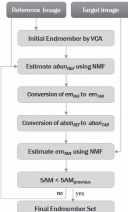
Fig. 1 shows the entire process of the endmember set estimation that we proposed. Each NMF unmixing updates the endmember sets or abundance maps of REF and TAR, which was done using multiplicative update rules as follows:
×
×
×
× ×
×
×
× ×
×
arccos ∥ 〈
∥ · ∥
〉 ∥
×
(3)
×
×
×
× ×
×
×
× ×
×
arccos ∥ 〈
∥ · ∥
〉 ∥
×
(4)
In Eqs. (3) and (4), em is either em
REFor em
TAR, and abun is either abun
REFor abun
TAR. IMG represents REF or TAR in each step. abun
Tand em
Tdenote the transposition of a matrix abun and em, respectively. em
iand abun
iare the em and abun in ith iteration step and can be updated to em
i+1and abun
i+1using Eqs. (3) and (4) (Berry et al., 2007).
The initial endmember set of REF for the fi rst NMF unmixing was estimated using vertex component analysis (VCA), which is an endmember extraction algorithm known for its fast processing in estimating the endmember spectrum in hyperspectral images (Nascimento and Bioucas-Dias, 2005). The initial ratio in each pixel of abun
REFwas 1 divided by the total number of endmembers. Eq. (4) was used with REF as IMG and abun
REFas abun to estimate abun
REFfi rst.
Then em
REFand the estimated abun
REFwere updated by Eqs. (3) and (4) where REF is IMG. The updated em
REFwas converted to em
TARby multiplying the spectral response function matrix between REF and TAR (BlackBridge, 2012). The updated abun
REFwas also converted to abun
TARby applying the point spread function by considering the spatial resolution of REF and TAR (Yokoya et al., 2012; Chi, 2013). The second NMF unmixing was performed using the converted em
TARand abun
TAR. At this time, em
TARwas updated by Eq. (3), where TAR was IMG and abun
TARis abun fi rst.
Then em
TARand the estimated abun
TARwere updated by Eqs.
(3) and (4), where REF is IMG. After the fi rst and second
NMF unmixing, the SAM value was estimated to measure
Fig. 1. Process of the endmember set estimation
the similarity of the updated em
REFand em
TAR. Because the SAM is insensitive to variations in illumination, it is effective to estimate the similarity of the updated em
REFand em
TARfrom images collected with different radiometric and atmospheric conditions. It uses the vector direction rather than the vector length. SAM becomes closer to zero as two images become spectrally similar. It can be calculated by Eqs. (5), where V
result1denotes the generic pixel vector element of the previous result and V
result2denotes the generic pixel vector element of the updated result. (Stathaki, 2008).
×
×
×
× ×
×
×
× ×
×
arccos ∥ 〈
∥ · ∥
〉 ∥
×
(5)
The second iteration process was performed by re-starting the fi rst NMF unmixing with the updated em
REF, not the initial em
REFestimated by VCA. The SAM value between the updated em
REFand em
TARdetermined from the second iteration process. This was compared with the SAM value estimated in the fi rst iteration process. If the current SAM value was smaller than the previous SAM value or the iteration loop reached a maximum number of iterations, the iteration loop was ended.
After the optimal endmember set between REF and TAR was estimated, band aggregation was performed based on the spectral response function of REF and TAR.
Using em
REFafter the band aggregation and em
TARfrom the optimal endmember set, we performed linear regression analysis and calibrated the TAR by applying estimated gain and offset to get calibrated result, TAR
calibrated, as follow:
×
×
×
× ×
×
×
× ×
×
arccos ∥ 〈
∥ · ∥
〉 ∥
×
(6)
3. Study Site and Data
The hyperspectral images collected by the airborne CASI- 1500 sensor were used to calibrate RapidEye multispectral images. The CASI-1500 sensor was developed by ITRES Research Ltd. of Canada. This sensor is a pushbroom imaging spectrometer with a spectrum ranging from 380 nm to 1050 nm. The CASI images used in this study were taken in the Sejong-bo area in Sejong-Ri Yeongi-Myun
Sejong-Si, Korea on 2 May 2014. Radiometric calibration, geometric correction, and optional environmental calibration were applied to collected stripes of CASI images to obtain orthocorrected images. RapidEye is a German geospatial information provider that operates fi ve observation satellites.
It is the fi rst commercial sensor to detect the Red Edge band and provides data with a spatial resolution of 5 m GSD at nadir.
The RapidEye scene for this study was collected at Sejong-si, including Sejong-bo, on 1 May 2014. The product level was 1B, which is radiometric- and sensor-corrected and provides imagery as seen from the spacecraft without correction for any geometric distortions inherent in the imaging process.
The specifi cations of the CASI and RapidEye images and the site scene are presented in Table 1, Fig. 2, and Fig. 3.
Table 1. Specifi cations of CASI and RapidEye images
Sensors CASI-1500 RapidEye
Spatial Resolution
(GSD) 1 m 5 m
Spectral Resolution
(nm)
48 Bands (363-1052)
Blue 440-510
Green 520-590
Red 690-730
Red Edge 630-685
NIR 760-850
Acquisition
Date 2014/05/02 2014/05/01
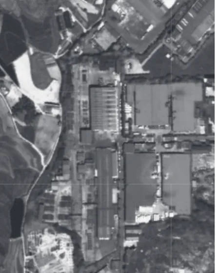
Fig. 2. Study site 1 displayed in 858.5 nm, 643.3 nm, and
557.2 nm as RGB channel
Registration between the CASI and RapidEye images was performed with manually collected GCPs. Study sites 1 and 2 were selected from areas that included water, vegetation, paddy fi elds, and urban structures.
In this study, the number of endmembers was set at 30.
The maximum number of iterations of the entire loop was fi ve because high numbers of the iteration of the entire loop caused abnormal abundance fractions because of the radiometric difference between the CASI and RapidEye images. The maximum number of iterations in individual NMF unmixing was set at 300 for optimal updating and appropriate time expenses. The threshold value to exit the individual NMF unmixing iteration by using Frobenius norm was set at 0.0001 (Yokoya et al., 2012).
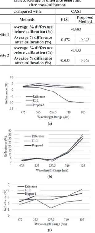
The results of the proposed cross-calibration method were compared with the results of empirical line calibration (ELC) utility in an ENVI program, which performed the cross-calibration with manually collected regions of interest (ROIs); 30 ROIs from the scene were collected manually from invariant features of urban structure, water, forest, paddy fi elds, and more to process the empirical line calibration. Both results were statically evaluated using the root mean square error (RMSE) and SAM to compare the pixel difference and spectral difference in the calibrated results with the reference data. The RMSE and SAM values
were calculated using Eqs. (7) and (5), respectively. In Eq.
(7), n is the total number of pixel, and reference (i) and result (i) are the refl ectance value of ith pixel in reference and result images, respectively. In Eq. (5), result 1 is reference and result 2 is the calibration result image. The average percent difference was also calculated to compare differences before and after cross-calibration. The average percent difference indicates the degree in percentage of the differences between the pixels in two images. It was calculated by Eq. (8), where reference is the matrix with refl ectance values of reference and result is the matrix with refl ectance values of calibration result (Chander et al., 2013).
×
×
×
× ×
×
×
× ×
×
arccos ∥ 〈
∥ · ∥
〉 ∥
×
(7)
×
×
×
× ×
×
×
× ×
×
arccos ∥ 〈
∥ · ∥
〉 ∥
×