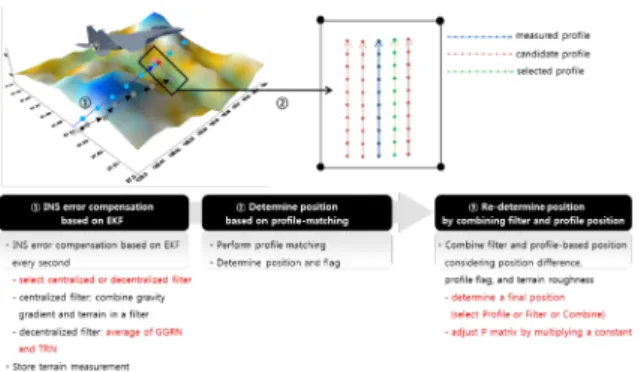
Development and Performance Analysis of a New Navigation Algorithm by Combining Gravity Gradient and Terrain Data as well as EKF and Profile Matching
11
0
0
전체 글
(2)
(3)
(4)
(5)
(6)
(7)
(8)
(9)
(10)
(11)
수치
+4
관련 문서
Research design, data, and methodology – The payment balance is a ratio of payment amounts made this country abroad and the receipts received by it from abroad for a
Changes in the composition and structure of Mediterranean rokey-shore communities following a gradient of nutrient enrichment: Descriptive study and test
As for the data used in this study, for the synoptic analysis, the surface weather chart and 500 hPa weather chart, which had been produced by the
Particularly, after selecting a specific cycle by collecting HWC data and primary system-related data from Gori NPP Unit 1 and comparatively analyzing
classifies data (constructs a model) based on the training set and the values (class labels) in a.. classifying attribute and uses it in
For the system development, data collection using Compact Nuclear Simulator, data pre-processing, integrated abnormal diagnosis algorithm, and explanation
Isostatic anomaly: the differences between reference data and observed data that went through latitude, free-air, bouguer, terrain and isostatic correction...
This study was performed by observation of the single nonwoven fabric filter bioreactors with the kind of nitrogen sources and conditional change by the
