1) 전북대학교 공과대학 토목/환경/자원에너지공학부 2) Hokkaido University
3) 한국지질자원연구원
* 교신저자 [email protected] 접수일 : 2021년 6월 7일 심사 완료일 : 2021년 6월 14일 게재 승인일 : 2021년 6월 21일
Abstract Recently, with the development of high-performance processing devices such as GPGPU, a three-dimensional dynamic analysis technique that can replace expensive rock material impact tests has been actively developed in the defense and aerospace fields. Experimentally observing or measuring fracture processes occurring in rocks subjected to high impact loads, such as blasting and earth penetration of small-diameter missiles, are difficult due to the inhomogeneity and opacity of rock materials. In this study, a three-dimensional dynamic fracture process analysis technique (3D-DFPA) was developed to simulate the fracture behavior of rocks due to impact.
In order to improve the operation speed, an algorithm capable of GPGPU operation was developed for explicit analysis and contact element search. To verify the proposed dynamic fracture process analysis technique, the dynamic fracture toughness tests of the Straight Notched Disk Bending (SNDB) limestone samples were simulated and the propagation of the reflection and transmission of the stress waves at the rock-impact bar interfaces and the fracture process of the rock samples were compared. The dynamic load tests for the SNDB sample applied a Pulse Shape controlled Split Hopkinson presure bar (PS-SHPB) that can control the waveform of the incident stress wave, the stress state, and the fracture process of the rock models were analyzed with experimental results.
Key words Three-dimensional dynamic fracture process analysis (3D-DFPA), Rock, Impact loading, Straight notched disk bending (SNDB), General-Purpose on Graphics Processing Units (GPGPU)
초 록 최근에는 GPGPU(General-Purpose computing on Graphics Processing Units)와 같은 고성능 연산장치의 보급과 함께 국방, 우주항공분야에서 암질재료에 대한 충격실험을 대신할 수 있는 3차원 동적해석기법의 개발이 활발하게 진행되고 있다. 그러나 높은 충격하중을 수반하는 암 발파 또는 소형미사일 등의 지중 관통과 같은 과정을 실험적으 로 관찰하거나 계측하는 것은 암질재료의 비 균질성 및 불투명성 때문에 어려움이 있었다. 본 연구에서는 고속충돌 에 의한 암석의 파괴 거동을 모사하기 위하여 3차원 동적 파괴 과정 해석 기법 (3D-DFPA)를 개발하였으며, 연산속 도를 향상시키기 위하여 순차해석(explicity analysis) 및 접촉요소검색(Searching algolitm of contact elements)에 GPGPU 연산이 가능한 알고리듬을 적용하였다. 제안된 동적파괴과정해석 기법에 대한 검증을 위해 Straight Notched Disk Bending (SNDB) 석회암시료에 대한 동적파괴인성시험을 모사하였고, 충격응력파의 전파과정, 암석-충격봉 경계면에 서 반사 및 전달과정, 암석 시료의 파괴과정을 비교분석하여, 개발된 해석기법에 대한 검증을 수행하였다.
핵심어 3차원 동적 파괴 과정 해석 기법 (3D-DFPA), 암질 재료, 충격 하중, Straight notched disk bending (SNDB), General-Purpose on Graphics Processing Units (GPGPU)
Development and Validation of the GPU-based 3D Dynamic Analysis Code for Simulating Rock Fracturing Subjected to Impact Loading
Gyeong-Jo Min1), Daisuke Fukuda2), Se-Wook Oh3), Sang-Ho Cho1)*1)
충격 하중 시 암석의 파괴거동해석을 위한 GPGPU 기반 3차원 동적해석기법의 개발과 검증 연구
민경조⋅Daisuke Fukuda⋅오세욱⋅조상호
1. Introduction
Evaluation of dynamic fracture toughness of rocks is of a significant importance in terms of understanding their resistances to external impact loads, such as percussive hammer drilling, small diameter missile penetration and explosive blasting, and to predict their fracturing behaviours for the achievement of optimum engineering designs.
However, in contrast to many static rock testing methods that are available, the number of established dynamic testing methods for the determination of dynamic fracture toughness of rocks is still limited.
For this purpose, one of the authors used the straight notched disk bend (SNDB) method for measuring dynamic fracture toughness of limestone (Cho et al., 2014). The work was motivated by the measurement of static fracture toughness of rocks using the SNDB method by Tutluoglu and Keles (Tutluoglu and Keles, 2011), as well as by the fact that the geometry of the SNDB sample is relatively simple and its shape is suitable to apply a split Hopkinson pressure bar (SHPB) test. The SNDB limestone samples were dynamically loaded and fractured under different loading rates using the SHPB system. The test results demonstrate that the limestone samples under the impact loading rate, 232 to 679 m/min, show the value of the dynamic fracture toughness ranging from 3.7 to 8.8 MN/m3/2, and the dynamic fracture toughness increases with respect to loading rate increment. However, many aspects of this mechanism have not been properly understood yet. Thus, the numerical simulation that would be able to realistically simulate the fracturing process in this test is essential. In our previous research, we proposed a two-dimensional finite-element-based dynamic fracture process analysis (2D-DFPA) code, which can simulate the problems of complex fracturing of rock−like materials under impact loadings, such as dynamic spalling (Cho et al., 2003), detonation-induced fracturing (Cho and Kaneko,
2004), and deflagration-induced fracturing (Fukuda et al., 2013). Spatial distribution of the microscopic strengths was used to consider rock inhomogeneity.
The fracturing was treated as separations of finite elements. Softening curve as a function of crack separation was employed to reflect the behaviour of the fracture process zone in front of the crack tips.
The code has been successfully applied to various dynamic fracturing problems, such as dynamic tension tests for rocks based on the spalling phenomena and dynamic fracturing of rock-like materials due to deflagration or detonation. However, 2D simulation is not a suitable option considering the sample geometry in the SNDB fracture toughness tests. In addition, since the dynamic loadings are applied by the SHPB system, not only the SNDB rock sample, but also the SHPB system must be modelled, which results in a significant increase of computational complexity. To overcome this problem, this paper presents the extension of the 2D-DFPA code to a three-dimensional version, which also uses Graphics Processing Unit (GPU) so as to significantly increase the capability of computational speed. Dynamic fracture of limestone subjected to impact loading based on the SNDB fracture toughness tests combined with the SHPB system was simulated by the 3D-DFPA. The validation of the code was performed by comparing the computational results, such as fracture patterns, stress profiles, and dynamic fracture toughness, with the experimental results.
2. GPU-based Three-dimensional Dynamic Fracture Process Analysis (3D-DFPA)
2.1 Theory of 3D-DFPA
The 2D-DFPA code previously developed by the present authors used an implicit 2D dynamic FEM for spatial discretization with the Newmark–β time integration scheme in which resulting simultaneous equation was solved by the Incomplete Cholesky Decomposition and Conjugate Gradient (ICCG)
scheme (Cho et al., 2003; Cho and Kaneko, 2004;
Fukuda et al., 2013). Although this approach may also be possible in the case of the 3D-DFPA code, the computational burden for the assemblage of large global matrix and solving the resulting simultaneous equation with the large number of degree of freedom would dramatically increase and the speed-up of the simulation requires quite a complex algorithm for parallel computation. Thus, the proposed 3D-DFPA code uses an explicit 3D dynamic FEM for spatial discretization with an explicit time integration scheme in which neither the assemblage of global matrix, nor the solution of large simultaneous equation is necessary. In addition, the explicit scheme is a promising approach for the efficient and easy-to-implement algorithm for parallel computation which will be described in the later sections.
Deformation of intact rock, i.e. the SNDB specimen, and metal corresponding to SHPB was modeled by the assembly of continuum solid elements, i.e. 4-node tetrahedral finite elements, in which isotropic neo-Hookean solid with viscous damping was assumed to be as follows (see Eq. (1)):
det det det (1)
where σij is Cauchy stress tensor; λ and μ, are the Lame’s constants; det(Fij), is the determinant of deformation gradient; δij, is the Kronecker delta; Eij, is the Green−Lagrange strain tensor; η, is the damping coefficient; Dij, is the rate of deformation tensor. By using the Green−Lagrange strain tensor, the large displacement and large rotation can be considered. Note that, in the range of stress level considered in this paper, Eq. (1) approximately corresponds to the isotropic liner elastic solid with viscous damping. In each tetrahedral finite element, Cauchy stress is converted to the equivalent nodal force fint for the explicit FEM. The fracturing process of rock, i.e. the opening and sliding of cracks, was
modelled using tensile and shear softening curves as a function of crack opening and sliding to reflect the behaviour of the fracture process zone in front of the crack tips and was expressed by 6-node initially zero-thickness cohesive elements (see Fig. 1). Normal and shear cohesive tractions acting on each cohesive element were computed using bi−linear tensile and shear softening models (see Fig. 2) depending on crack opening displacement (COD) and crack sliding (Slip), respectively. The microscopic shear strength was computed by the Mohr-Coulomb model with tension cut−off. By following the concept of the 2D DFPA code, the microscopic tensile strength and microscopic cohesion of each cohesive element were determined using Weibull’s distribution (see Eq.(2)).
exp
(2)
where Γ is a Gamma function; m, is a coefficient of uniformity; V, is a volume characterized by the size of each tetrahedral element; Vref, is a reference volume characterized by the size of rock specimen;
and St(Vref), is a mean microscopic tensile strength or microscopic cohesion in Vref. In the implementation of the 3D DFPA code, random numbers satisfying Eq.
(2) were generated to give first the spatial distribution of St(V) for each tetrahedral element. Then, the microscopic tensile strengths and the microscopic cohesion of each cohesive element were calculated by taking the average of its surrounding tetrahedral elements’ values of strengths. Application of Eq. (2) is equivalent to considering material heterogeneity and the size effect of strength characterized by m and the ratio of V to Vref, respectively. Internal friction angle was assumed to be constant. When the critical values of COD or Slip were achieved in a cohesive element, the cohesive element was deactivated and its surfaces were considered as new rock surfaces, i.e. macro fracture surfaces. The cohesive elements were inserted into all the boundary of the tetrahedral elements
corresponding to rock at the beginning of the analysis. It is worth noting that the method adopted here is categorized into the so-called intrinsic cohesive zone model (Zhang et al., 2007) where the initial elastic behaviour of the cohesive elements for 0<COD< CODEL and 0<Slip< SlipEL must be also prescribed (see Fig. 2) in which CODEL and SlipEL
are the elastic limits of COD and Slip, respectively.
The values of CODEL and SlipEL are inversely proportional to a normal crack penalty, Pn, and a tangential crack penalty, Ptan, respectively, and, in order to avoid the spuriously large compliance of the cohesive elements, these should be sufficiently small.
Therefore, Pn and Ptan can be considered as the stiffness of the cohesive element for Mode I and
Mode II deformation and should ideally be infinity to achieve elastic behavior which is accordance with that for the surrounding tetrahedral elements, while this requires the infinitesimal time step. Since this is impossible in the actual numerical simulation, sufficiently large values of Pn and Ptan compared to the Young’s modulus of rock were used as a compromise. As shown in Fig. 2, we also considered loading/unloading in each cohesive element. In addition, when the negative COD occurs, repulsive force is applied in order to cancel the negative COD in which the large value of Pn is used for the stiffness. In each cohesive element, the normal and shear cohesive tractions are converted to the equivalent nodal force fcoh for the explicit FEM.
Fig. 1. 6-node cohesive element used in the 3D-DFPA inserted between all the tetrahedral elements corresponding to rock. The initial thickness of all the cohesive elements is initially zero.
Fig. 2. Treatment of opening (Left) and sliding (Right) behaviors of cracks based on tensile/shear softening.
The contact processes between the material surfaces including the contact between the newly created macro fractures by separation of each cohesive element were modelled by the penalty method (Munjiza, 2004). In this method, when the tetrahedral elements on the material surface were in contact with each other, the overlapped shape formed by the overlapping tetrahedral elements was exactly computed and the contact force, which is proportional to the area of the overlapped surface with the proportionality coefficient PDEM, was computed for each contacting couple. The dynamic friction between the contact surfaces was also considered based on Coulomb’s friction law. Contact detection algorithm is described in 2.2. In each contacting couple, the contact force is converted to the equivalent nodal force fcon for the explicit FEM. Based on the aforementioned procedures, the following equation of motion, which can be solved explicitly with respect to time, was obtained in the framework of explicit FEM (see Eq. (3)):
(3)
where Mlump is a lumped mass matrix; u, the nodal displacement; fext, the nodal force corresponding to the external load which is given by the analysist.
Courant-Friedrichs-Lewy (CFL) condition must be satisfied for the convergence of analysis, resulting in the requirement of a very small time step. There are various possibilities for the explicit time integration scheme for Eq. (3), such as the central difference (CD), the bulk viscosity method, the Chung-Lee, the Hulbert, the Newmark, the Nor-Bathe, the Tchamwa-Wielgosz (TW), and the Zhai. (Nor and Bathe, 2013; Maheo et al., 2013). Among these techniques, we employed the TW explicit time integration scheme, because its implementation is simple, can effectively reduce the spurious oscillation, and requires a single-step algorithm, i.e. computationally
efficient, although it is first-order accurate. It is worth mentioning that we also tried some of the aforementioned time integration techniques, including the CD scheme, in the developing stage of the 3D-DFPA; however, we often encountered the numerical instability even for a smaller time step.
2.2 Application of GPGPU to 3D-DFPA
For the achievement of a significant speed-up of simulation by the 3D-DFPA, we incorporated a parallel computation scheme based on the NVIDIA®
Tesla® K20 graphics processing unit (GPU) accelerator (NVIDIA, 2013) into the 3D-DFPA code.
The computation on GPU was controlled through the NVIDIA’s CUDA® architecture by CUDA Fortran (Ruetsch and Fatica, 2013), which is essentially Fortran 90 with several extensions that make it possible to leverage the power of GPUs in the computations. A greater degree of parallelism occurs within the GPU itself. Subroutines that run on the GPU are executed by many threads in parallel.
Although all threads execute the same code, these threads typically operate on different data. This data parallelism is called the “fine-grained parallelism”, in which it is most efficient to have adjacent threads operate on adjacent data, such as elements of an array (Ruetsch and Fatica, 2013). It is not uncommon to have the number of resident threads on a GPU in an order of magnitude larger than the number of cores on the GPU. In the K20 GPU accelerator used in the current DFPA code, the number of processor cores is 2496 (NVIDIA, 2013).
Thus, a higher computational performance can be achieved, as compared to ordinary CPUs. In the framework of the CUDA programming model, a serial code is executed by many GPU threads in parallel. Each thread executing this code has a means of identifying itself in order to operate on different data; however, the code that CUDA threads execute is very similar to the serial CPU code, which is one
of the advantages of the application of CUDA, while the code of many parallel CPU programming models, such as Message Passing Interface (MPI), greatly differs from the serial CPU code.
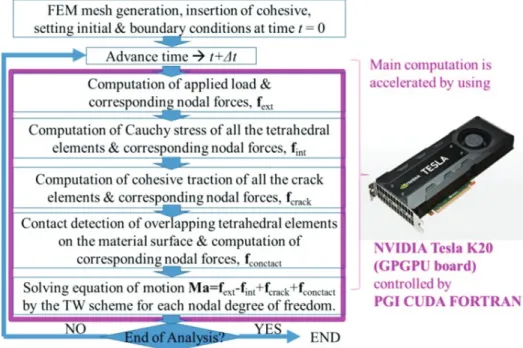
In Fig. 3, a flowchart of the 3D-DFPA using the GPU is shown. Since the GPU device is controlled by the CPU in the CUDA programming model (Ruetsch, 2011), all the data, including the FEM mesh, initial and boundary conditions, are first generated by the CPU in the RAM in the host computer, i.e. not in the memory on the GPU device.
Then, all the data are transferred from the RAM in the host computer to the memory in the GPU device.
It is worth mentioning that the data transfer between the host computer and the GPU device is rather slow and, therefore, the minimization of the data transfer is the key to success of the drastic speed-up by the use of GPU. Data transfer from the GPU to the host computer is always necessary for the outputting the analysis results. In the implementation of the 3D DFPA code, computations for fext, fint in each tetrahedral element, fcoh in each cohesive element, fcon
in each contacting couple, and nodal degree of freedom in Eq. (3) were assigned to each core of the GPU device and processed in a massively parallel manner. However, one of the challenging problems was the achievement of the efficient contact detection for identifying each contacting couple only through the GPU. For example, in the case of sequential CPU implementation, the No Binary Search (NBS) contact detection algorithm (Munjiza, 2004) can achieve the linear search in which the required computation for the contact detection is proportional to the number of targets for contact detection.
However, such contact detection algorithm cannot be applied to the GPU implementation. Therefore, we used the alternative approach. First, we subdivided the analysis domain comprising a massive number of target tetrahedral elements into multiple equal-sized cubic sub-cells so that the largest target tetrahedron in the model was completely included in a single sub-cell. In this way, every target tetrahedral element can have a corresponding single sub-cell to which it belongs. By using integer coordinate for the location
Fig. 3. Flowchart of the 3D DFPA using a GPGPU board.
of each sub-cell and by assigning unique hash values to the integer coordinate of each sub-cell, the element ID data for all the target tetrahedral elements were sorted according to the hash values as key. Thus, for each sub-cell, the IDs of all the tetrahedral elements included in each sub-cell can be readily available in this method. For the key-sorting by hash, the radix sorting algorithm optimized for CUDA (Satish et al., 2009) was used. Finally, for a particular cell, only searching its adjacent 27 cells for contact detection was sufficient and this made it possible to achieve efficient contact detection only on the GPU.
Therefore, the 3D DFPA can run in a completely parallel on the GPU and no sequential processing is necessary, except for the input and output procedures.
3. SNDB fracture toughness test combined SHPB system
Fig. 4 shows a schematic diagram and a photo of a SNDB limestone sample. The mode-I dynamic fracture toughness KIC−D of the SNDB sample is calculated as follows (see Eq. (4)):
(4)
where a is the initial notch length, R is the radius of the specimen, t is the thickness of the specimen, Pcr is the maximum compressive force applied to the SNDB at failure, YISNDB is a dimensionless stress intensity factor. YISNDB is expressed by YISNDB = m(S/R)+n with m and n depending on t/R and a/t
ratios. The values of m and n are determined by the line fitting. For the target limestone, the values of a, R and t were 4 mm, 18.5 mm and 20 mm, respectively. Thus, approximate values of m and n were 5.9 and 0.42, respectively, resulting in the YISNDB
= 3.4 (Tutluoglu and Keles, 2011). The aperture of the notch was 1 mm.
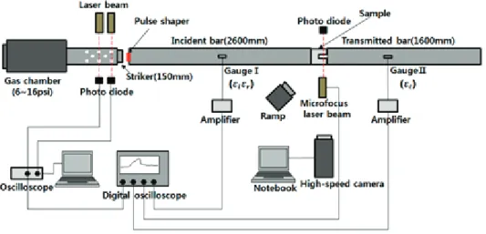
The SHPB system was used to dynamically load the SNDB limestone sample. Fig. 5 shows a schematic illustration of the SHPB system which consists of a striker bar, an incident bar, a transmitted bar, and a data acquisition system. Two semi−conductor strain gauges are mounted in the middle of the incident bar and the transmitted bar.
The SNDB limestone sample was sandwiched by specially manufactured jigs attached on the surfaces of the incident bar and the transmitted bar. By accelerating the striker bar by the gas gun and letting it collide with one end of the incident bar, approximately 1D compressive stress wave is induced by the impact and it starts to propagate towards the SNDB sample. The pulse shaping technique was employed to achieve dynamic stress equilibrium and constant strain rate through the test sample before the sample failure. Some portion of the stress wave reflects at the contacting face between the incident bar and the rock sample, while the remaining portion of it transmits into the rock. The transmitted stress wave in the rock further propagates towards the transmitted bar, and reflection and transmission of the stress wave occurs again when the stress wave arrives at the interface between the rock and the
Fig. 4. Schematic illustration and photo of a SNDB limestone sample.
transmitted bar.
As such, the SNDB rock sample is subject to dynamic 3-point bending, resulting in the splitting of the rock into two halves. In this literature (Cho et al., 2014) and this paper, the time history of strain in transmitted bar was converted to the applied loads, P, by using Young’s modulus and cross-sectional areas of the transmitted bar. Thus, Pcr was computed as the maximum value of P and dynamic fracture toughness was calculated using Eq. (4). A strain gauge mounted on the incident bar and transmitted bar measured the incident pulse (εi), reflect the pulse (εr) and transmitted pulse (εt). Based on the
one-dimensional elastic wave propagation theory with the assumption of homogeneous deformation of the specimen, the forces on both ends of the specimen can be calculated as follows (see Eq. (5)-(7)):
(5)
(6)
(7)
where A is the cross section area and E is the elastic modulus of the bar. Pav(t) is the average load of specimen. The fracture process was observed by
Fig. 5. Schematic illustration of SHPB system.
(a) LS2 (b) LS5
Fig. 6. Strain–time histories measured on the incident and transmitted bars in the LS2 and LS5 tests
high-speed video camera. Fig. 6 shows strain–time histories measured on the incident and transmitted bars in the LS2 and LS5 tests. The results of SNDB fracture toughness tests are summarized in Table 1.
Sample No.
Loading rate (mm/min)
Max.
Load Pcr (kN)
Critical stress (MPa)
KIC-D
(MN m3/2)
LS1 376800 26.84 18.14 7.00591
LS2 448800 26.17 17.68 6.82942
LS3 547200 26.83 18.13 7.00125
LS4 586200 29.64 20.02 7.73492
LS5 661800 28.88 19.52 7.53828
LS6 654600 33.12 22.38 8.64314
LS7 307800 24.38 16.47 6.363
LS8 679800 32.19 21.75 8.40007
LS9 515400 31.38 21.21 8.1905
Table 1. Summary of the SNDB dynamic fracture toughness test results
4. Numerical model and anaysis condition for DFPA
4.1 Model description
The numerical model for the 3D-DFPA of SNDB limestone sample subjected to dynamic load by SHPB is shown in Fig. 4. The model considers the exact shape of the SNDB sample and the SHPB system.
The cohesive elements were inserted to all boundaries of tetrahedral elements corresponding to the portion
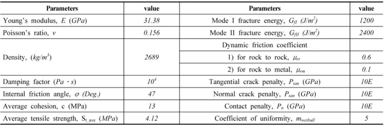
of limestone, and not to the portion of the metal bars. Since the possible crack paths are only along the boundaries between each tetrahedral element in the DFPA, this requires a very fine mesh for realistic crack propagation and a considerable amount of computation is necessary. The total number of the nodes, the tetrahedral elements, and the cohesive elements were 1449343, 395310, and 707840, respectively, and it is clear that these numbers are considerably large for the sequentially implemented CPU code. A single NVIDIA Tesla® K20c GPGPU accelerator was used. As shown in Fig. 7, the fitting curve of experimentally recorded stress wave profile in the incident bar was applied to an end of the incident bar corresponding to the velocity of striker bar, vstriker= 8.6 m/s. The physical properties of limestone were set as shown in Table 2. In the Table 2, E, ν, ρ, φ, c and St_ave were experimentally determined, while other values were assumed. The DFPA was conducted with the time step of Δt = 10-9 s.
The incident stress waveforms obtained from the tests listed in Table 1 were used as applied pressure-time history on the start end of the incident bar in the 3D-DFPA model. Fig. 8 shows the temporal change of axial stress for the incident bar and the transmitted bar, respectively, which were obtained from both the strain gages and the 3D-DFPA. Note that t = 0 in the Fig. 8 indicates
Fig. 7. Numerical model for the 3D DFPA of the SNDB limestone sample subjected to dynamic load by SHPB
the arrival of the stress wave at the measuring points in the incident bar and the transmitted bar. By comparing these results, considering the noise included in the experimental results, the DFPA results show a relatively good agreement with the experimentally obtained stress wave profiles. For the incident wave, the DFPA slightly overestimates the amplitude of reflected wave, while the shapes of the waves show a good agreement. It is worth noting that the interface between the specially manufactured jigs and incident/transmitted bars are taped together by plastic tape in the experiment, while the DFPA model in this paper assumed that the interface was exact
continuum. Thus, specifically in the case of reflection wave, some contact damping could occur between the interface in the experiment and, thus, DFPA that does not consider this interface effect, could simulate its amplitude rather large as compared to the experiment. Another reason could due to the assumption of zero-damping in the incident bar and the transmitted bar. For the transmitted wave, DFPA slightly underestimates the amplitude of reflected wave, while the shapes of the waves yield a good agreement. The difference could be due to the rough estimate of the fracture energy used in this paper;
therefore, further investigation will be necessary in
Parametersvalue Parameters value
Young’s modulus, E (GPa) 31.38 Mode I fracture energy, GfI (J/m2) 1200 Poisson’s ratio, v 0.156 Mode II fracture energy, GfII (J/m2) 2400
Density, (kg/m3) 2689
Dynamic friction coefficient
1) for rock to rock, μrr 0.6 2) for rock to metal, μrm 0.1
Damping factor (Paㆍs) 104 Tangential crack penalty, Ptan (GPa) 10E
Internal friction angle, φ (Deg.) 47 Normal crack penalty, Ptan (GPa) 10E
Average cohesion, c (MPa) 13 Contact penalty, Pn (GPa) 10E
Average tensile strength, St_ave (MPa) 4.12 Coefficient of uniformity, mweibull 5 Table 2. Physical properties of limestone used for the 3D-DFPA
(a) Incident bar (b) Transmitted bar
Fig. 8. Calculated stress wave profile for the incident bar and the transmitted bar
our future task. Fig. 9 compares the experimental fracture toughness and calculated fracture toughness by using the 3D-DFPA. The calculated fracture toughness increased with the increase of the strain rate. A high correlation between the experimental and numerical fracture toughness was observed. This means that the 3D-DFPA can simulate the strain rate dependency of fracture toughness without any incorporation of the strain rate dependency model.
Fig. 9. Numerical model for the 3D-DFPA of the SNDB limestone sample subjected to dynamic load by SHPB.
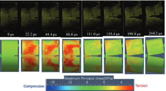
4.2 Verification of numerical simulation results Fig. 10 shows a comparison of the fracture processes by the high-speed video camera and by the 3D-DFPA for a selected time. In the DFPA result, the color in the limestone part means the spatial distribution of the maximum principal stress where tension is shown in warm color. It is clear that mode-I fracture occurs along the center of the specimen from the notch tip towards the incident bar and the crack mouth opening displacement gradually increases with respect to time. It is also notable that high tensile stresses are also found in the region between the roller jigs and impactor jig, although no significant fracturing occurs in these parts. The experiment results and the DFPA at t = 244.2 μs agree well in terms of the macro fracture pattern and crack mouth opening displacement.
By assuming that the interface stresses on both ends of the limestone specimen are uniform, the stress on the transmission bar can be used to obtain the maximum compressive force, Pcr, in Eq.(4). In this case, Pcr can be computed by the maximum value of stress profile in Fig. 8(b) and cross−sectional area of the transmitted bar. The dynamic stress intensity
Fig. 10. Fracture processes photographed by a high-speed video camera and simulated by the GPU–based 3D DFPA.
factor, KIC-D, corresponding to the experiment and the DFPA is 7.15 MN/m3/2 and 6.13 MN/m3/2, respectively. Again, considering the noise included in the experiment, the aforementioned interface effect and the difference of the detail of the microstructure between the actual limestone and the DFPA model, the difference of KIC-D seems to be rather acceptable;
therefore, it can be concluded that the applicability of the 3D-DFPA code is validated.
4.3 Influence of the loading rate on the dynamic fracture toughness
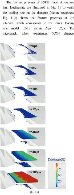
The fracture processes of SNDB model at low and high loading-rate are illustrated in Fig. 11 to verify the loading rate on the dynamic fracture toughness.
Fig. 11(a) shows the fracture processes at 2μs intervals, which corresponds to the lowest loading rate model (LS1), within 20μs – 26μs. The microcrack, which experiences 0-25% damage,
(a) LS1 (b) LS8
Fig. 11. Distribution of fracture process zone around notch tip
propagates and the front of the microcracks are almost flat. The macro cracks, which corresponds to open cracks, appear after 84μs. Figure 11(b) shows the fracture processes for a model that corresponds to the highest loading rate model (LS8) at 2 μs intervals within 6 μs - 12μs. When compared with Fig. 11(a), the microcracks in the centre area are slower. According to Cho et al. (2003), the decreased crack velocity at higher loading rates increases the dynamic tensile strength of rock. Thus, the micro crack propagation velocity decreased at higher loading rate, leading to higher dynamic fracture toughness.
5. Conclusion
This paper explained the newly developed three-dimensional Dynamic Fracture Process Analysis (3D-DFPA) code utilizing GPGPU. Dynamic fracture of limestone subjected to impact loading based on the Straight Notched Disk Bending (SNDB) fracture toughness tests combined with the split Hopkinson pressure bar (SHPB) system was simulated by the 3D-DFPA. The validation of the code was conducted by comparing the numerical results with those obtained by the experimently in terms of the fracture pattern, stress profile, and dynamic fracture toughness. The simulated fracture pattern showed a quite good agreement with the experimentally obtained one. For the stress wave profile and dynamic fracture toughness, although the slight difference was observed between the DFPA and experimental results, the shape of the stress wave was expressed quite well. Thus, it may be possible that the dynamic fracture toughness could be predicted by the 3D-DFPA code with some proper calibrations.
Since only one loading pattern was simulated in this paper, our future task is to apply the 3D-DFPA to various loading patterns and to validate our code in more detail. One of the important implications in this paper is that the introduction of only a “single”
GPU in a small workstation can obtain the results
shown here within several “hours”, while the sequential CPU–based simulation needs “dozens of days” to complete the same simulation. Since the application of multiple GPUs is possible and can be introduced with a relative ease and at a relatively lower cost, further drastic speed–up could be possible in future research, where more detailed fracture simulations will be realized.
Acknowledgments
This work is supported by the Korea Agency for Infrastructure Technology Advancement(KAIA) grant funded by the Ministry of Land, Infrastructure and Transport (Grant 21CTAP-C164314-01).
References
1. Cho, Sang Ho, Katsuhiko Kaneko, 2004, Influence of the applied pressure waveform on the dynamic fracture processes in rock, Int J Rock Mech Min Sci, Vol. 41, No. 5, pp. 771-784.
2. Cho, Sang Ho, Yuji Ogata, Katsuhiko Kaneko, 2003, Strain-rate dependency of the dynamic tensile strength of rock, Int J Rock Mech Min Sci, Vol. 40, No. 5, pp. 763-777.
3. Cho, SH, HM Kang, MS Kim, H Eustache, M Kataoka, Y Obara, and K Xia, 2014, Determination of Dynamic Fracture Toughness of Rocks using Straight Notched Disk Bending (SNDB) Specimen, ISRM International Symposium-8th Asian Rock Mechanics Symposium.
4. Fukuda, Daisuke, Kazuma Moriya, Katsuhiko Kaneko, Katsuya Sasaki, Ryo Sakamoto, and Keitaro Hidani, 2013, Numerical simulation of the fracture process in concrete resulting from deflagration phenomena, Int J Fract, Vol. 180, No. 2, pp. 163-175.
5. Maheo, Laurent, Vincent Grolleau, and Gérard Rio, 2013, Numerical damping of spurious oscillations: a comparison between the bulk viscosity method and the explicit dissipative Tchamwa–Wielgosz scheme, Computational Mechanics, Vol. 51, No. 1, pp. 109-128.
6. Munjiza, Antonio A., 2004, The combined finite- discrete element method, John Wiley & Sons.
7. NVIDIA, 2013, TESLA K20 GPU accelerator board specification.
8. Ruetsch, Greg, and Massimiliano Fatica, 2011, Cuda
fortran for scientists and engineers, NVIDIA Corporation.
9. Satish, Nadathur, Mark Harris, and Michael Garland, 2009, Designing efficient sorting algorithms for manycore GPUs, 2009 IEEE International Symposium on Parallel & Distributed Processing.
10. Tutluoglu, Levent, Cigdem Keles, 2011, Mode I fracture toughness determination with straight notched
disk bending method, Int J Rock Mech Min Sci, Vol.
48, No. 8, pp. 1248-1261.
11. Zhang, Zhengyu, Glaucio H Paulino, and Waldemar Celes, 2007, Extrinsic cohesive modelling of dynamic fracture and microbranching instability in brittle materials, Int J Numer Methods Eng, Vol. 72, No. 8, pp. 893-923.
민 경 조
전북대학교 공과대학 토목/환경/자원에너지공학부 박사과정
Tel: 063-270-4636 E-mail: [email protected]
Daisuke Fukuda Hokkaido University, Faculty of Engineering Assistant Professor
Tel: 063-270-4636
E-mail: [email protected]
오 세 욱
한국지질자원연구원 지질환경연구본부 심지층연구센터 선임연구원
Tel: 042-868-3178 E-mail: [email protected]
조 상 호
전북대학교 공과대학
토목/환경/자원에너지공학부 교수
Tel: 063-270-4636 E-mail: [email protected]