Effect of Grid Cell Size on the Accuracy of Dasymetric Population Estimation
Byong-Woon JUN
1※격자크기가 밀도구분적 인구추정의 정확성에 미치는 영향
전병운
1※*
ABSTRACT
This study explored the variability in the accuracy of dasymetric population estimation with different grid cell sizes. Dasymetric population maps for Fulton County, Georgia in the US were generated from 30m to 420m at intervals of 30m using an automated intelligent dasymetric mapping technique, population data, and original and simulated land use and cover data. The accuracies of dasymetric population maps were evaluated using RMSE and adjusted RMSE statistics. Lumped fractal dimension values were calculated for the dasymetric population maps generated from resolutions of 30m to 420m using the triangular prism surface area (TPSA) method. The results show that a grid cell size of 210m or smaller is required to estimate population more accurately in terms of thematic accuracy, but a grid cell size of 30m is required to meet an acceptable spatial accuracy of dasymetric population estimation in the study area. The fractal analysis also indicates that a grid cell size of 120m is the optimal resolution for dasymetric population estimation in the study area.
KEYWORDS : Population, Dasymetric Estimation, Scale, Resolution, Fractal
요 약
본 연구는 상이한 셀 크기에 따라 밀도구분적 인구추정의 정확성이 어떻게 변화하는지를 탐색하 였다. 미국 조지아주 풀턴 카운티를 사례로 한 밀도구분적 인구 지도가 지능적인 밀도구분적 지도 제작기법, 인구자료, 원본 및 모의된 토지이용 및 피복 자료를 이용하여 30m에서 420m의 해상도 까지 매 30m 간격으로 생성되었다. 밀도구분적 인구 지도의 정확성은 RMSE 및 수정 RMSE 통 계치를 이용하여 평가되었다. 프랙털 차원 값은 TPSA 방법을 사용하면서 30m에서 420m의 해상
2016년 9월 4일 접수 Received on September 4, 2016 / 2016년 9월 26일 수정 Revised on September 26, 2016 / 2016년 9월 27일 심사완료 Accepted on September 27, 2016
1 경북대학교 지리학과 Department of Geography, Kyungpook National University
※ Corresponding Author E-mail : [email protected]
도까지 생성된 밀도구분적 인구 지도에 대해 각각 계산되었다. 연구결과에 따르면, 속성의 정확성 측면에서 인구를 보다 정확하게 추정하기 위해서 210m 이하의 격자 셀 크기가 적절하였나, 사례 지역에서 밀도구분적 인구추정의 허용가능한 공간적 정확성을 충족시키기 위해 30m의 격자 셀 크 기가 적절하였다. 또한, 프랙털 분석은 120m의 격자 셀 크기가 사례지역에서 밀도구분적 인구추 정을 위한 최적의 해상도 이다는 것을 보여준다.
주요어 : 인구, 밀도구분적 추정, 스케일, 해상도, 프랙털
INTRODUCTION
Data about the size and geographic distribution of populations are necessary for investigating urban issues such as crime, public health, hazard assessment, emergency response, service accessibility, environmental justice, and so on (Landford, 2006; Liu and Herold, 2007; Higgs and Landford, 2009; Choei, 2010; Patino and Duque, 2013). Using the spatial population data, improved population estimates can be obtained as the base data for further analysis.
Although census data are ready to use, it is inappropriate to directly use the census data for these environmental and socio- economic applications mentioned above since the data are usually aggregated up to the administrative units due to the privacy issue and do not provide information on the spatial distribution of people within the administrative units. Even the census data suffered from the modifiable areal unit problem (MAUP), which is a long-standing problem with spatial data analysis (Openshaw, 1983).
Dasymetric population estimation method, which utilizes the ancillary data on the spatial distribution of populations such as land use and land cover data derived from remotely sensed images, has been widely used for these environmental and socio-
economic applications in an urban area because this method provides a relatively accurate and stable population estimate among other population estimation methods (Wu et al., 2005). The term ‘dasymetric’
denotes‘density measuring’in the English dictionary. The dasymetric population estimation method with remotely sensed images can be grouped into two categories such as dasymetric mapping and regression modeling approaches(Langford, 2006). The dasymetric mapping approach originally developed by Wright(1936) redistributes populations into sub-zones within the administrative units relying on the ancillary data about their geographic distribution.
The regression modeling approach infers population counts based on the regression relationship between populations and their correlates such as urban areas, land use and cover, dwelling units, image pixel characteristics, and other physical or socio- economic characteristics(Wu et al., 2005).
According to spatial resolution, there are three types of the ancillary data for use in dasymetric population estimation in support of these applications(Wu et al., 2005;
Cockx and Canters, 2015). Urban and
non-urban areas are roughly used as the
low-resolution ancillary data. Land use and
land cover data are the most commonly
used as the medium-resolution ancillary
data while local data on street networks,
building, parcels(Maantay et al., 2007), and addresses are seldomly adopted as the high-resolution ancillary data depending on the data availability. This study is limited to the dasymetric mapping approach with land use and land cover as the medium-resolution ancillary data.
Until recently, multi-resolution land use and cover data ranging from 1m to 1km have been used for dasymetric population mapping at different spatial scales ranging from local to regional to global scales (Dobson et al., 2000; Eicher and Brewer, 2001; Mennis, 2003; Bozheva et al., 2005;
Langford, 2006; Gallego et al., 2011;
Goerlich and Cantarino, 2013; Cockx and Canters, 2015). Despite the wide-spread use of dasymetric population mapping, few studies have been concerned with investigating the effect of grid cell size or spatial resolution on the accuracy of dasymetric population mapping(Eicher and Brewer, 2001; Mennis, 2003; Bozheva et al., 2005; Hultgren, 2005; Wu et al., 2005;
Langford, 2006). Although some of them have addressed theoretically the possible impacts of grid cell size on the accuracy of dasymetric population mapping and the optimal spatial resolution needed to map populations effectively(Eicher and Brewer, 2001; Mennis, 2003; Wu et al., 2005;
Langford, 2006), few empirical studies have been pronounced by far and have even shown contrasting results with the land use and land cover data derived from remotely sensed images ranging from 1m to 48m(Bozheva et al., 2005; Hultgren, 2005). The dasymetric population mapping using remotely sensed imagery as the ancillary data is not free from MAUP. It is still not clear that to what degree the grid
cell size may over or underestimate populations and what the optimal spatial resolution is for representing populations with dasymetric mapping. This issue has not been exhaustively scrutinized in the international research community for urban analysis and modeling.
In this context, this study explores how the accuracy of dasymetric population estimation changes with different grid cell sizes in Fulton County, Georgia in the US.
Unlike the previous studies, this study uses land use and land cover data as the medium-resolution ancillary data ranging from 30m to 420m and a fractal analysis to find the optimal grid cell size or spatial resolution for dasymetric population mapping.
The existing literature pertaining to dasymetric population mapping and MAUP is reviewed in the next section. Data and methods used in this study are described in the following section. The results obtained from this study are then presented and some issues to be considered are discussed.
In the final section, concluding comments are addressed.
DASYMETRIC POPULATION MAPPING AND MAUP
One of the special issues about spatial
data analysis is MAUP originally addressed
by Openshaw(1983). There are two
dimensions of MAUP. One is the scale
effect which refers to the variability in
analytical results caused by data collected
at different geographic scales or different
levels of spatial resolution for the same
area. The other is the aggregation or
zoning effect which denotes the variability
in analytical results generated by data
collected from different zonal systems with the same number and extent of areal units. The effect of MAUP is usually applied to zonal vector data, but this can be conceptually and practically extended to raster data(Wong, 1996; Usery et al., 2004; Wu et al., 2008). The dasymetric population mapping using remotely sensed images is thus tied up with the effect of MAUP.
Some previous studies have theoretically attempted to explore the effect of grid cell size or spatial resolution on the accuracy of dasymetric population mapping. By reviewing the spatial resolution requirements of remotely sensed data for urban studies, Jensen and Cowen(1999) suggested that the spatial resolution of remotely sensed images required for local population estimation in urban settings would be 0.25m to 5m whereas that for regional and national population estimation would be 5m to 20m.
Eicher and Brewer(2001) addressed the possible impacts of grid cell size on the accuracy of dasymetric population mapping and mentioned the need to determine the optimal grid cell size for dasymetric population mapping over diverse map scales considering accuracy, storage requirement, and processing time. Mennis(2003) also pointed out that one should balance computation time with accuracy and take account of the spatial variation of population distribution in an urban area in order to find out the optimal grid cell size for dasymetric population mapping. Wu et al.(2005) reviewed the previous studies related to population estimation methods using relatively coarse resolution satellite images and then expected the potential of very high resolution commercial satellite
images such as QuickBird and IKONOS in improving the accuracy of dasymetric population estimation as demonstrated in Liu(2003)’s study. Langford(2006) brought attention to the issue of the optimal spatial resolution required to represent populations effectively with dasymetric mapping.
Few empirical studies have focused on examining the effect of grid cell size or spatial resolution on the accuracy of dasymetric population mapping. Bozheva et al.(2005) investigated the effect of spatial resolution on the accuracy of dasymetric population mapping using land cover data derived from remotely sensed images such as airborne color infrared images in 1m, ASTER images in 15m, a Landsat 7 ETM+ panchromatic image in 15m, and Landsat 7 ETM+ multi-spectral images in 30m for Black Hawk County, Iowa in the US. They used a binary class method including residential/non-residential areas for dasymetric population mapping. They demonstrated that the accuracy of dasymetric population mapping would tend to increase with higher levels of spatial resolution. In contrast, Hultgren(2005) examined the role of spatial resolution in dasymetric population mapping using land use and land cover data extracted from remotely sensed images such as IKONOS multi-spectral imagery in 4m and the aggregated images in 8m, 12m, 16m, 24m, 32m, and 48m for north Denver, Colorado in the US. In his study, a three-class method including high-density residential, low-density residential, and others was used for dasymetric population mapping.
He suggested that the spatial resolution
appropriate for dasymetric population
mapping might be from 10m to 20m and
the spatial resolution had an inconsistent effect on the accuracy of dasymetric population mapping. Further, he addressed that the method properties and the resolution of population source had a little more effect on dasymetric population mapping than the spatial resolution of the ancillary data.
Some theoretical studies have clearly indicated the need to study the impacts of grid cell size on the accuracy of dasymetric population mapping and to find the optimal grid cell size for representing populations effectively. However, two empirical studies have showed contrasting results with either the binary-class or the three-class method and the ancillary data ranging from 1m to 48m in different study areas. Eicher and Brewer(2001) and Langford(2006) demonstrated that the choice between the binary class and the three-class method in dasymetric population mapping provided inconsistent results. Although multi-resolution land use and land cover data reaching from 1m to 1km have been adopted for dasymetric population mapping so far, multi-resolution land use and land cover data spanning from 48m to 1km have not been used to investigate the effect of MAUP on the outcome of dasymetric population mapping.
There has been no empirical research into finding the optimal grid cell size or spatial resolution in dasymetric population mapping.
Many studies have also argued that the classification accuracy of the ancillary data would be important in dasymetric population mapping(Martin et al., 2000; Bozheva et al., 2005; Langford, 2006; Jun, 2006) though some studies have not supported with the finding(Fisher and Langford,
1996; Hultgren, 2005; Wu et al., 2005).
The effect of classification accuracy on dasymetric population mapping has not been systematically investigated by now to seek for the optimal grid cell size. This and other issues are under the rubric of the effect of MAUP on dasymetric population mapping.
DATA AND METHODS
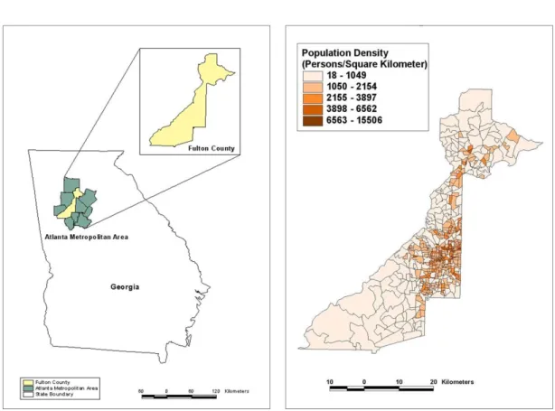
In this study, Fulton County, Georgia in the US was selected as a study area as shown in Figure 1. The study area is located at the core part of the Atlanta metropolitan area, which is one of the fast growing and suburbanizing metropolitan areas in the US. This study area was chosen considering its data availability and the spatial variation in population distribution. The population density in 2000 as depicted in Figure 2 illustrates that the population distribution is spatially varied in the study area.
The primary data sets for this research include population data from 2000 US Census and land use and cover data derived from 2000 Landsat 5 TM imagery.
The demographic data were collected at the census tract and block group levels.
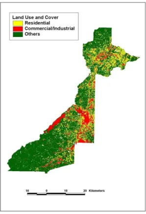
The land use and cover data were initially
extracted from the Landsat imagery using
a hybrid digital image classification and
then reclassified into three classes such
as residential, commercial/industrial, and
others as shown in Figure 3. The land use
and cover data have a spatial resolution of
30m and an overall classification accuracy
of 86.7%. To simulate different spatial
resolutions, the land use and cover data
were resampled into 60m to 420m at
FIGURE 1. Location of study area
FIGURE 2. Population density intervals of 30m using the nearest
neighborhood method, respectively. The nearest neighbor method was used in the resampling process because the land use and land cover data belong to nominal data and the resampling method keeps the original pixel values unchanged. The original and simulated multi-resolution land cover and land use data ranging from 30m to 420m were finally adopted for dasymetric population mapping because the spatial resolutions for the ancillary data between 48m and 1㎞ have not been used to measure the effect of MAUP on dasymetric population mapping by far.
Dasymetric population maps were generated from 30m to 420m at intervals
of 30m using an automated intelligent dasymetric mapping (IDM) technique. The IDM estimates the population count for a given target zone taking the source population data as input count data and the original and simulated land use and land cover data as categorical ancillary data.
The equation for the IDM suggested by Mennis and Hultgren(2006) is given as follows:
∈
(1)
where A
tis the total area for target zone
t, D
cis the estimated density of ancillary
class c, within a given source zone, y
sis
the resident population count for source
FIGURE 3. Land use and land cover zone s, and y
tis the population estimate
for target zone t. The IDM redistributes the source population data into sub-zones within the administrative units on the basis of an integrated approach of areal weighting and empirical sampling methods to determine the relative densities of each ancillary class(Mennis and Hultgren, 2006).
There are three sampling methods such as containment, centroid, and percent cover methods. In this study. the percent cover sampling method(with 70 percent) was used for a reliable IDM parameterization. The entire IDM process was automated and implemented in ArcGIS 10.1 environment by a python script originally developed by Mennis and Hultgren(2006), revised by Sleeter and Gould(2007), and last updated
by Sleeter and Gould in 2014. The python script was ultimately modified as necessary for use in this study. For this study, population data and IDM parameterization were controlled while different grid cell sizes or levels of spatial resolution was experimented in order to explore the effect of MAUP on dasymetric population mapping.
The accuracies of the 14 dasymetric
population maps were evaluated using the
root mean square error(RMSE) and the
adjusted RMSE statistics. The RMSE and
the adjusted RMSE statistics are calculated
using the following equations (Fisher and
Langford, 1995; Gregory, 2002):
(2)
(3)
where n is the total number of census zones, z
iis the resident population count for census zone i, and u
iis the population estimate for census zone i. The RMSE introduced by Fisher and Langford(1995) statistically quantifies the error involved with dasymetric population mapping. The adjusted RMSE suggested by Gregory(2002) minimizes the unexpected consequences caused by a census zone with larger RMSE.
These two statistics were used in this study because these are readily applicable to count data and it is easy to interpret their results(Hawley and Moellering, 2005;
Jun, 2006).
A fractal analysis was implemented to measure the scale change and to find the optimal grid cell size or spatial resolution in dasymetric population mapping(Lam, 1992; Cao and Lam, 1997; Wong et al., 1999). Lumped fractal dimension values were calculated for the dasymetric population maps generated from resolutions of 30m to 420m at intervals of 30m using the triangular prism surface area(TPSA) method. The TPSA method was selected in this study due to its relative accuracy and applicability to surfaces with higher spatial complexity in comparison to other methods such as isarithm and variogram methods(Lam et al., 2002; Zhou and Lam, 2005). The fractal dimension values were quantified using the image characterization
and modeling system (ICAMS) software package (Quattrochi et al., 1997).
RESULTS AND DISCUSSION
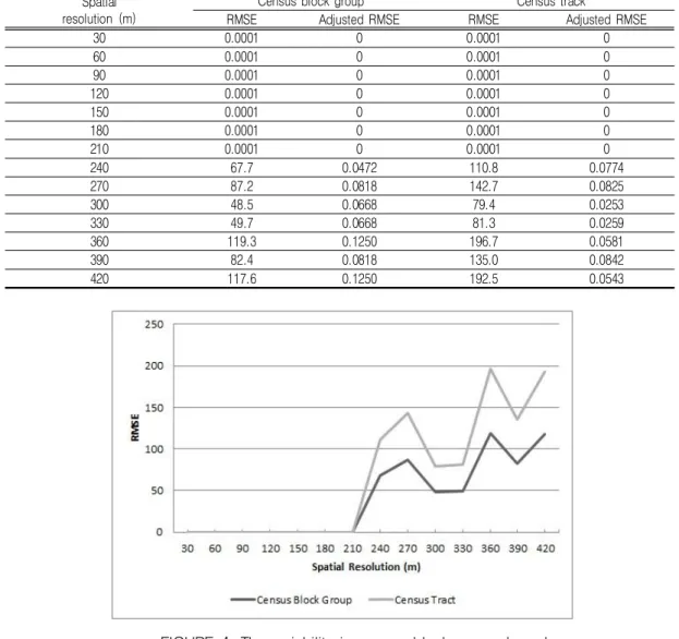
The thematic accuracies of 14 resultant dasymetric population maps were quantified by the RMSEs and the adjusted RMSEs.
The RMSEs and the adjusted RMSEs were measured by cross validation. For cross validation, the dasymetric population maps were aggregated up by census block group and census tract and then the aggregated population estimates were compared with the actual populations for the census zones.
Two source population data such as the actual populations for census block groups and census tracks were used for dasymetric population mapping in this study. Census block group is the smallest census zone with various demographic and socio- economic data in the US while census track is made up of multiple census block groups.
Table 1 shows the RMSEs and the adjusted RMSEs introduced by the 14 dasymetric population maps when the actual populations for census block groups were used as source population data. FIGURE 4 shows the variability in the RMSEs and the adjusted RMSEs of the 14 dasymetric population maps with different grid cell sizes or levels of spatial resolution.
The RMSEs and the adjusted RMSEs of
the 14 dasymetric population maps are
close to zero from 30m to 210m,
regardless of the census zones for
aggregation in cross validation. The RMSEs
and the adjusted RMSEs aggregated by
census block group repeat to increase and
decrease inconsistently within the range of
120 from 240m to 420m while those
Spatial resolution (m)
Census block group Census track
RMSE Adjusted RMSE RMSE Adjusted RMSE
30 0.0001 0 0.0001 0
60 0.0001 0 0.0001 0
90 0.0001 0 0.0001 0
120 0.0001 0 0.0001 0
150 0.0001 0 0.0001 0
180 0.0001 0 0.0001 0
210 0.0001 0 0.0001 0
240 67.7 0.0472 110.8 0.0774
270 87.2 0.0818 142.7 0.0825
300 48.5 0.0668 79.4 0.0253
330 49.7 0.0668 81.3 0.0259
360 119.3 0.1250 196.7 0.0581
390 82.4 0.0818 135.0 0.0842
420 117.6 0.1250 192.5 0.0543
TABLE 1. Census block group-based RMSEs and adjusted RMSEs
FIGURE 4. The variability in census block group-based RMSEs and adjusted RMSEs by spatial resolution aggregated by census track fluctuate
within the range of 200. The RMSEs and the adjusted RMSEs tend to get higher when the dasymetric population maps were aggregated up by census tract rather than by census block group. This is the reason why high-resolution population data from census block groups were
down-scaled to low-resolution population data from census tracks.
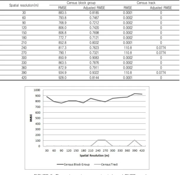
Table 2 represents the RMSEs and the
adjusted RMSEs caused by the 14
dasymetric population maps when the
actual populations for census tracts were
used as source population data. Figure 5
illustrates how the RMSEs and the
Spatial resolution(m) Census block group Census track
RMSE Adjusted RMSE RMSE Adjusted RMSE
30 883.5 0.8185 0.0001 0
60 793.8 0.7467 0.0002 0
90 768.9 0.7212 0.0002 0
120 806.0 0.7420 0.0002 0
150 806.8 0.7698 0.0002 0
180 772.7 0.7121 0.0002 0
210 852.8 0.8032 0.0001 0
240 817.3 0.7623 110.8 0.0774
270 790.1 0.7321 110.8 0.0774
300 850.9 0.9083 0.0002 0
330 863.5 0.7876 0.0002 0
360 872.9 0.7911 0.0002 0
390 934.9 0.9322 110.8 0.0774
420 928.0 0.8144 0.0001 0
TABLE 2. Census tract-based RMSEs and adjusted RMSEs
FIGURE 5. The variance in census tract-based RMSEs and adjusted RMSEs by spatial resolution
adjusted RMSEs of the 14 dasymetric population maps are varied when different grid cell sizes were used.
The RMSEs and the adjusted RMSEs aggregated by census block group change from 768 to 935 with different grid cell sizes. This case shows much higher errors because low-resolution population data
from census tract were up-scaled to
high-resolution population data from
census block group. The RMSEs and the
adjusted RMSEs aggregated by census
tract are close to zero from 30m to 210m,
from 300m to 360m, and at 420m while
these reach to around 111 from 240m to
270m and at 390m.
Spatial resolution(m) Fractal dimension
Census block group Census track
30 2.2357 2.1940
60 2.3182 2.3201
90 2.3186 2.3279
120 2.3450 2.3876
150 2.3269 2.3286
180 2.4526 2.4403
210 2.4316 2.4116
240 2.4257 2.5538
270 2.4886 2.5718
300 2.5118 2.5670
330 2.4908 2.4801
360 2.4909 2.4962
390 2.5680 2.5510
420 2.5246 2.5657
TABLE 3. Fractal dimension values by spatial resolution The RMSEs and the adjusted RMSEs
are relatively lower when the census zone for source population data is the same as that for aggregation in cross-validation as shown in Table 1 and Table 2. For instance, a combination of census block group and census block group or census tract and census tract results in the lower errors.
The errors are likely to be relatively lower when a combination of census block group and census block group is used because census block group provides higher-resolution population data than census tract. When a combination of census tract and census tract is used, the errors tend to be averaged out. The overall results from the thematic accuracy assessment show that a grid cell size of 210m or smaller provides the lowest error for dasymetric population mapping in this study.
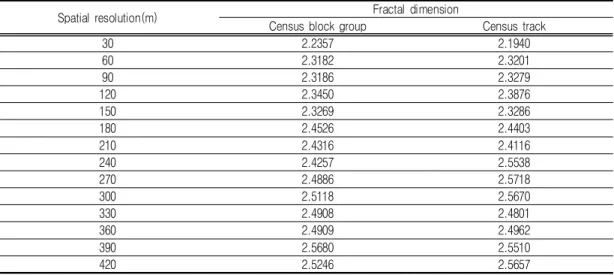
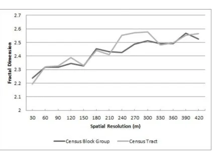
Table 3 and Figure 6 show the change of the fractal dimension values calculated for the 14 dasymetric population maps with different grid cell sizes. In this study, a fractal analysis was used to characterize
the change in scale and to determine the optimal grid cell size for dasymetric population mapping. Typically, fractal dimension values range from 2.0 to 3.0 for a surface. The change of fractal dimension values over scale indicates the change in the scale at which geographic phenomena operate(Lam, 1992; Cao and Lam, 1997; Wong et al., 1999; Moon, 2005). The highest fractal dimension value measured across scale sheds light on the scale at which most of the geographic phenomena under consideration operate (Lam, 1992; Cao and Lam, 1997). In this way, one can determine the optimal grid cell size for dasymetric population mapping.
Since the thematic accuracy assessment
identified that the spatial resolution
required for dasymetric population mapping
in this study was a grid cell size of 210m
or smaller, the fractal analysis placed a
special focus on the spatial resolutions
from 30m to 210m. The fractal dimension
values for census block group and census
track steadily increase from 30m to 120m,
FIGURE 6. The variability of fractal dimension values by spatial resolution
turn to decrease at 150m, and then repeat to go up and down from 180m to 210m.
There are two turning points at 120m and 180m within the range of 210m. These turning points suggest the spatial resolutions at which the scale change emerges. The first turning point at 120m is selected as the optimal grid cell size or spatial resolution for dasymetric population mapping in this study though the second turning point at 180m shows the higher fractal dimension values because fractal dimension values show a steady increase by the turning point and after that there appear several significant turns indicating the scale change.
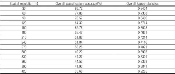
The IDM technique used in this study employes land use and land cover data as ancillary data. The classification accuracy of land use and land cover data has some effect on the accuracy of dasymetric population mapping(Martin et al., 2000;
Bozheva et al., 2005; Langford, 2006; Jun, 2006). It is necessary to measure the
effect of classification accuracy on the accuracy of dasymetric population mapping.
Table 4 represents the variability in the classification accuracies of land use and land cover data by spatial resolution. The overall classification accuracies of multiple -resolution land use and land cover data steadily decrease from 30m to 420m. The overall classification accuracy of the original land use and land cover data in 30m was degraded from 86.72% to 35.68%
by the resampling method used in this study. These overall classification accuracies were correlated with the RMSEs as shown in Table 1 and Table 2 in order to measure the effect of classification accuracy on the accuracy of dasymetric population mapping.
The correlation coefficients calculated for census block group and census tract in Table 1 are –0.76. This indicates that the higher the classification accuracy of land use and land cover data, the higher the accuracy of dasymetric population mapping.
The correlation coefficient for census
Spatial resolution(m) Overall classification accuracy(%) Overall kappa statistics
30 86.72 0.8404
60 77.86 0.7338
90 70.57 0.6466
120 64.32 0.5714
150 62.76 0.5528
180 55.47 0.4651
210 51.82 0.4214
240 51.04 0.4116
270 50.26 0.4021
300 49.22 0.3905
330 44.27 0.3301
360 44.53 0.3338
390 41.93 0.3041
420 35.68 0.2265