Linear controller design for the longitudinal model of a reusable launch vehicle X-33

1. INTRODUCTION

For the several decades, the reduction of the cost and capable replacement for the U.S. space shuttle motivated the application of next generation reusable launch vehicles (RLVs). Those triggered the design and the development of the X-33 vehicle which includes the following main features, the linear aerospike engine, vertical take-off, horizontal landing and aerodynamic configuration[1]. The X-33 is a wedged-shaped subscale technology demonstrator prototype of a potential future Reusable Launch Vehicle (RLV) that Lockheed Martin has dubbed VentureStar[2].

In the dynamic behavior's point of view, X-33 is designed to travel at a top speed of Mach 15 and, in addition, its transfer function model includes the initial value term which inevitably effects on transient response. Therefore it is recommended to find a controller such that X33 has a fast and well damped time responses under the given environments. This implies that we are to find a controller which meets both tracking performance and surpassing of the initial value effects.

In this paper, a linear controller is designed for the longitudinal model of X-33 in TAEM (The Terminal Area Energy Management) phase by using CRA. As the design method, the characteristic ratio assignment (CRA) is introduced to deal directly with the overshoot and speed of step response of an all-pole system of arbitrary order. The method is based on certain relationships between characteristic polynomial coefficients and transient responses.

The paper consists of the following four sections. In section 1, the introduction with the main purpose of the paper is given. In section 2, an analysis on X-33 is applied and brief mathematical theories on CRA are derived. After showing the main results in section 3 followed by some simulations in section 4, the conclusive remarks are added in section 5.

2. X-33 MODEL DESCRIPTION AND CRA

In this section, after the brief introduction to X-33, the transfer function model of X-33 is developed from the given state-space equations. The description of the plant includes that of an actuator. Also some preliminaries on CRA, the design method in this paper, are briefly described.

2.1 Basic configuration of X-33 in TAEM phase

Fig. 1 shows a typical early X-33 vehicle and its surfaces. The surfaces include body flaps at the outboard engine locations, inboard and outboard elevons on the canted fins, and two rudders on the vertical tails. The X-33 vehicle was designed to use an aerospike engine, which allows for pitch and roll thrust vectoring as well as differential thrust yaw control. Also the dynamics of X-33 considerably depends on the flight conditions.

In this paper, the Terminal Area Energy Management (TAEM) phase, one of three major phases which are to be encountered during the flight of the X-33 vehicle, is considered as the landing phase. TAEM phase begins when the vehicle is slowed to mach 3. Also the region of flight can exhibit areas of instability and need to be controlled by an acceleration command controller.

2.2 Longitudinal model description of the X-33 vehicle The linearized state-space equations for the longitudinal plant model of X-33 are given by

Fig. 1 Typical X-33 configuration

Linear controller design for the longitudinal model of a reusable launch vehicle

X-33

Youngtae Woo*, Jaejin Kim

**

and Youngchol Kim

***

* Department of Electronic Engineering, Chungbuk University, Cheong-ju, Korea (Tel : +82-43-261-2475; E-mail: wytnice@chungbuk.ac.kr)

** Department of Electronic Engineering, Chungbuk University, Cheong-ju, Korea (Tel : +81-43-261-2475; E-mail: wowlsl@chungbuk.ac.kr)

***School of Elec. & Computer Eng., Chungbuk National Univerity, Cheong-ju, Korea (Tel : +81-43-261-2475; E-mail: yckim@cbu.ac.kr)

Abstract: In this paper, a linear controller is designed for the longitudinal model of X-33 in TAEM (The Terminal Area Energy Management) phase. The CRA (Characteristic Ratio Assignment) is used as the continuous time design method such that the output response of X-33 control system tracks the reference command. The performance of the proposed controller is evaluated through the step response. Also simulation results show that the initial state of the plant is dominantly affected by the poles and zeros of the plant.

⎥ ⎥ ⎥ ⎥ ⎥ ⎦ ⎤ ⎢ ⎢ ⎢ ⎢ ⎢ ⎣ ⎡ ⎥ ⎥ ⎦ ⎤ ⎢ ⎢ ⎣ ⎡ − ⎥ ⎦ ⎤ ⎢ ⎣ ⎡ ⎥ ⎥ ⎦ ⎤ ⎢ ⎢ ⎣ ⎡ = ⎥ ⎦ ⎤ ⎢ ⎣ ⎡ fl fr lm rm fl fr l r fl fr l r q M M M M V Z V Z V Z V Z q M M V Z q δ δ δ δ α α δ δ δ δ δ δ δ δ α α ₁ & & ₍₁₎ ⎥ ⎥ ⎥ ⎥ ⎥ ⎦ ⎤ ⎢ ⎢ ⎢ ⎢ ⎢ ⎣ ⎡ ⎥ ⎦ ⎤ ⎢ ⎣ ⎡ − ⎥ ⎦ ⎤ ⎢ ⎣ ⎡ ⎥ ⎥ ⎥ ⎦ ⎤ ⎢ ⎢ ⎢ ⎣ ⎡− = ⎥ ⎦ ⎤ ⎢ ⎣ ⎡ fl fr lm rm r r r r g z Z Z Z Z q s Z q N δ δ δ δ α δ δ δ δ α 0 0 0 0 2 . 32 1 1 0 0 ₍₂₎

whereNzis a normal acceleration,

α

is an angle of attack

(rad),qis pitch body rate(rad/sec),

δ

_in=

[

δ

_rm

δ

_lm

δ

_fr

δ

_fl

]

are control inputs and the rest of symbols are moment aerodynamic coefficients. In this paper, all control inputs of

δ

_inare assumed to the same. Therefore the plant has SIMO structure of one input and two output system. From (1) and (2), the transfer function with no initial values can be derived as

04154 . 0 17015 . 0 27626 . 0 09532 . 0 53455 . 0 ) ( ) ( ) ( ₂ 2 1 1 _{+ +} − − − = = s s s s s D s N s G p (3) 04154 . 0 17015 . 0 00025111 . 0 033587 . 0 ) ( ) ( ) ( 2 ₂ 2 + + + = = s s s s D s N s G p (4)

HereinG1(s)is for the angle of attack andG2(s)for pitch

body rate. Also the model of actuator is given as follows:

3993 . 696 9451 . 36 39901 ) ( ) ( ) ( ₂ + + = = s s s D s N s G a a a (5)

In addition, with the initial values, the model description of the plant including actuator can be expressed by

) 0 ( ) ( ) ( ) ( ) ( ) ( ) 0 ( ) ( ) ( ) ( ) ( 1 3 1 1 1 α α s D s N s U s D s N s H s U s G s Y p + = + = (6) ) 0 ( ) ( ) ( ) ( ) ( ) ( ) 0 ( ) ( ) ( ) ( ) ( 2 4 2 2 2 α α s D s N s U s D s N s H s U s G s Y p + = + = (7) where

D

(

s

)

=

D

p

(

s

)

D

a

(

s

)

, ) ( ) ( ) ( ₁ 1 s G s G s G = _a , G₂(s)=G_a(s)G₂(s), ) 162 . 0 ( 0082 . 0 ) ( 3 s =− s− N , 04 . 0 ) ( 4 s =Mα=− N .

Also

α

(0)denotes the initial value. Box B in Fig. 5 represents the model of the plant which includes the actuator.

Thus, the main purpose of this paper is to design a linear controller such that the output responses of longitudinal control system of X-33 track the reference command as rapid as possible with small overshoot and the stability of the closed-loop system is maintained.

2.3 Definitions

Let us consider a real characteristic polynomial as follows:

.

0

.

)

(

1 0 1 1

+

+

+

∀

>

+

=

− − i n n n n

s

a

s

a

s

a

a

a

s

_L

δ

(8)

The characteristic ratios are defined as

n n n n a a a a a a a a a 2 2 1 1 3 1 2 2 2 2 0 2 1 1: , : , , : − − − = = =

α

α

α

_L , (9)

and the generalized time constant is defined as

0 1 : a a =

τ

. (10)

The coefficientsa_iof

δ

(s)may also be represented in terms of

α

_i’s and

τ

as follows:

τ

0 1 a a = , (11) . , , 3 , 2 , 1 1 2 2 3 3 2 2 1 0 _{i n} a a _{i i} i i i i i L L = = _{− −} − − −

α

α

α

α

α

τ

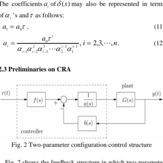
(12) 2.3 Preliminaries on CRA

Fig. 2 Two-parameter configuration control structure

Fig. 2 shows the feedback structure in which two-parameter configuration is occupied. It is the control structure which has the advantages in that it allows a minimal realization of system and does not increase zeros of overall system. From Fig. 2, the transfer functions of the closed loop system are expressed by ) ( ) ( ) ( ) ( ) (sY s n s f s R s P = (13) ) ( ) ( ) ( ) ( ) (s d sa s n sb s P = + (14) For the purpose of satisfactory time response to the given linear plant model, the main procedure of CRA can be summarized as follows:

i) First, find a desired *

(

)

s

δ

by means of

α

i’s and

τ

.

ii) In full order case, obtain the feedback controller gains of

a

(s

)

and

b

(s

)

by solving the Diophantine equation

)

(

)

(

)

(

)

(

)

(

*

s

s

b

s

n

s

a

s

d

+

=

δ

.

iii) Determine the feed-forward gains of

f

(s

)

to compensate the effect of zeros and accuracy.

Example 1[3]: Consider the two parameter configuration for

controller structure shown in Figure 2. Let us consider a sixth-order unstable plant with poles at −1.2± j3 ,

2 2 . 3 ± j

− , 2± j2and zero initial conditions:

s s s s s s s s s d s n s G 27 . 213 02 . 65 232 . 11 84 . 12 8 . 4 ) 5 . 2 ( 600 ) ( ) ( ) ( 2 3 4 5 6 2 + + + + + + + = = =

and let the controller polynomials be:

0 0 1 2 2 3 3 4 4 5 5 0 1 2 2 3 3 4 4 5 5 ) ( ) ( ) ( f s f b s b s b s b s b s b s b a s a s a s a s a s a s a = + + + + + = + + + + + =

Suppose that the objective is to design a feedback controller such that the closed loop step response has no overshoot and a 1% settling time of 1 sec.

We let ) 5 . 2 )( ( ) (_s =_{a s s}2+_s+ a , _n(_s)=_n(_s)(_s2+_s+2.5) .

Then, the closed loop equation can be written as

)

(

)

(

)

(

)

(

)

(

:

)

(

s

p

s

n

s

f

s

R

s

Y

s

T

=

=

where

)

5

.

2

)(

(

)

(

)

(

)

5

.

2

)(

(

)

(

)

5

.

2

)(

(

)

(

2 2 2

+

+

+

+

+

=

=

+

+

=

s

s

s

n

s

b

s

d

s

s

s

a

s

a

s

s

s

p

s

p

(15)

In (15), p(s)of order 9 should be chosen by the CRA method. Then the overall system will be an all-pole one. In order to obtain a properp(s), we first set

τ

=1. To illustrate this, we choose the following three

α

₁’s:

[

2 2.1 2.25

]

1=

α

Then using (11) and (12), the desired polynomials are constructed. For convenience, we lety_i(t),

i

=

1

,

2

,

3

be the step response of theT_i(s)whereT_i(s),

i

=

1

,

2

,

3

is the all pole system with

α

₁=

[

2 2.1 2.25

]

, respectively. As shown in Fig. 3 and summarized in table 1, no overshoot is achieved at

α

₁=2.25.

Fig. 3 Step response of desired closed loop systems with various

α

₁s

Table 1 Percentage overshoot with respect to

α

₁values

1

α

2 2.1 2.25

overshoot in % 17.12% 2.26% ≈0%

From this analysis, we select

α

1=2.25. Next we compute

the appropriate value of

τ

such that the desired speed is achieved. From the step responsey₃(t), the 1% settling time (the time required to reach 99% to the steady state value) is shown as 1.914 sec. Here we have

52246 . 0 ) 1 ( 914 . 1 1 1 1 2 ⋅ = ⋅ = =

τ

τ

t t sec. Finally, 1500 ) ( 3 . 1495 74 . 782 7 . 181 466 . 24 0527 . 2 098911 . 0 ) ( 9407 . 5 525 . 2 4379 . 2 06035 . 0 10 587 . 8 10 3989 . 5 ) ( 2 3 4 5 2 3 4 4 5 6 = + + + + + = + + + + × + × = − − s f s s s s s s b s s s s s s a

and Fig. 4 shows that the design is achieved successfully.

Fig. 4 Step response of desired closed loop systems with various

α

1=2.25

From the above results, it is evident that for a given set of values ofα ,is τ anda0, the corresponding polynomial,

δ

(s),

is completely described. Kim [3] has shown that the generalized time constant is precisely related to the speed of system response. An important result is that the speed of response of a linear all-pole system can be controlled, while maintaining the exact shape of response, by adjusting the value of

τ

if itsαisare the same.

3. LINEAR CONTROLLER DESIGN

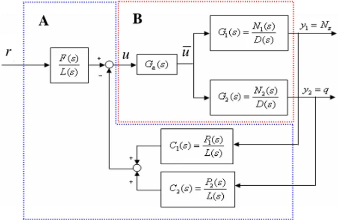
In this section, we design the continuous time linear controllers for (6) and (7) using the CRA. The order of the proposed controller in each loop is equal to 3. Box A in Fig. 5 shows the proposed control structure in which two-parameter configuration is occupied. The structure avoids the effect of adding ‘zero’ to overall transfer function the closed loop.

Fig. 5 Block Diagram of controllers for X-33

In Fig. 5, the model blocks are denoted by the following symbols: Plant 1: ) ( ) ( ) ( 1 1 s D s N s G = Plant 2: ) ( ) ( ) ( 2 2 s D s N s G = Actuator: ) ( ) ( ) ( s D s N s G a a a =

A

B

u

u

r

Controller 1: 0 1 2 2 3 10 11 1 1 ) ( ) ( ) ( a s a s a s b s b s L s P s C + + + + = = Controller 2: 0 1 2 2 3 20 21 2 2 ) ( ) ( ) ( a s a s a s b s b s L s P s C + + + + = = Pre-filter: 0 1 2 2 3 0 ) ( ) ( a s a s a s f s L s F + + + =

where

γ

is reference signal,y₁is normal acceleration andy₂is pitch body rate. Then, the transfer functions of the closed loop system is expressed by ) 0 ( ) ( ) ( ) ( ) ( ) ( ) ( ) ( ) ( ) ( ) ( ) ( ) ( ) ( ) ( ) ( 4 1 2 3 2 2 3 1 α s s D s N s N s P s N s N s P s N s D s L s R s s F s Y p ∆ − + + ∆ = (16) ) 0 ( ) ( ) ( ) ( ) ( ) ( ) ( ) ( ) ( ) ( ) ( ) ( ) ( ) ( ) ( ) ( ) ( ) ( 4 2 1 4 1 1 4 1 2 2 α s s D s N s N s P s N s N s P s N s D s L s R s s N s F s N s Y p ∆ − + + ∆ = (17) where ). 10 25 . 0 28 . 0 93 . 28 ( ) 10 25 . 0 03 . 0 28 . 0 10 . 0 93 . 28 03 . 120 ( ) 03 . 0 10 . 0 53 . 0 93 . 28 03 . 120 73 . 702 ( ) 93 . 28 53 . 0 03 . 120 73 . 702 12 . 37 ( ) 03 . 120 73 . 702 12 . 37 ( ) 73 . 702 12 . 37 ( ) 12 . 37 ( ) ( ) ( ) ( ) ( ) ( ) ( ) ( 20 3 10 0 21 3 20 11 10 1 0 2 21 11 10 2 1 0 3 11 2 1 0 4 2 1 0 5 2 1 6 2 7 2 2 1 1 b b a s b b b b a a s b b b a a a s b a a a s a a a s a a s a s s N s P s N s P s D s L s − − × + − + × + + − − + + + − − + + + + − + + + + + + + + + + + + = + + = ∆

Next, we set the target polynomial of the overall system. By using (9) and (10), the polynomial can be generated. Therefore, we make the following target polynomial by selecting

3000 0= a ,

α

₁=2.75,

τ

=2[sec]. 4371 . 232033 87 . 464066 18 . 337503 14 . 114803 8 . 19653 39 . 1693 24 . 68 ) ( 2 3 4 5 6 7 * + + + + + + + = ∆ s s s s s s s s (18)

Then the controller gains are determined from the algebraic relation between∆(s)and *

(

)

s

∆

as follows: 22 . 3769 57 . 164 12 . 31 12 . 360 03 . 131 ) ( ) ( ) ( 1 _{3 2} 1 _{+ − +} − = = s s s s s L s P s C (19) 22 . 3769 57 . 164 12 . 31 78 . 38 23 . 1900 ) ( ) ( ) ( 2 _{3 2} 2 _{+ − +} − − = = s s s s s L s P s C (20)

Also pre-filter gainf₀is determined as 232033.44.

Fig. 6 Closed-loop response ofN_z

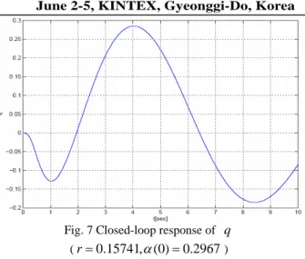
Fig. 7 Closed-loop response of q

(r=0.15741,

α

(0)=0.2967)

4. SILMULATIONS RESULTS

With the designed controllers in (19) and (20), the proposed controller’s ability to track the reference input and performance are evaluated through some simulations. Fig. 6 shows the output responses ofN_zto the reference command.

The results from Fig. 6 show that the proposed controller is designed such that X-33 vehicle system has no overshoot with a relatively high undershoot and the effect of nonzero initial values on the output responses exists. In addition, a larger time constant

τ

of CRA is needed to be set for a relatively small undershoot. It implies that the output response of X-33 control system is slow to track the reference command. However, if the initial states are all zeros, the proposed controller provides the non-overshooting step response as well as very quick response time. Also Fig. 7 shows the output response ofq.

5. CONCLUSIONS

For the longitudinal control of the X-33 vehicle, a linear controller is designed in TAEM (The Terminal Area Energy Management) phase by using CRA. The models of X-33 are described as transfer functions for the output feedback control.

The results show that the plant has inherently slow modes because the poles of the plant and zeros are located at near origin. This implies that even though the target characteristic polynomial is selected in fast mode to track the reference command as rapidly as possible, the effect of the initial state is dominantly affected by the poles and zeros of the plant. Also the assumption that all control inputs are the same is one of the reasons which disable the improvement of performance of X-33 control system.

Therefore, it can be said that it is not possible to avoid nonzero initial condition problems as long as a linear controller is applied. However, with non initial condition, the proposed controller gives rise to a good transient response and non-overshooting output response. To overcome the limitation of the performance specification, an alternative control scheme is considered in the future research.

ACKNOWLEDGMENTS

This research was supported by grant CN-055 from the Program for the Training of Graduate Students in Regional Innovation which was conducted by the Ministry of Commerce Industry and Energy of the Korean Government.

REFERENCES

[1] Philip, C., “An Entry Flight Controls Analysis for a Reusable Launch Vehicle,” AIAA Paper 2000-1046, Jan. 2000.

[2] Lockwood, M., “Overview of Conceptual Design of Early VentureStarTM Configurations,” AIAA Paper 2000-1042, Jan. 2000.

[3] Y. C. Kim, L. H. Keel, and S. P. Bhattacharyya, “Transient Response Control via Characteristic Ratio Assignment,” IEEE Trans. On Automatic Control, vol. AC-48, no.12, pp.2238-2244, DEC. 2003.

[4] G. F. Franklin, J. D. Powel, and A. Emani-Naeini,

Feedback Control of Dynamic Systems, Prentice-Hall,

Upper Saddle River, New Jersey, 2002.

[5] S. Manabe, “Coefficient diagram method,” in Proceedings of the 14th IFAC Symposium on Automatic Control in Aerospace, pp.199-210, Seoul, Korea, 1998.