Prediction of Extreme Sloshing Pressure Using Different Statistical Models

Journal of Advanced Research in Ocean Engineering 4(4) (2018) 185-194

http://dx.doi.org/10.5574/JAROE.2018.4.4.185

Prediction of Extreme Sloshing Pressure

Using Different Statistical Models

Ekin Ceyda Cetin

_{, Jeoungkyu Lee}

_{, Sangyeob Kim}

_{, and Yonghwan Kim}

1_{Department of Naval Architecture & Ocean Engineering, Seoul National University, Seoul, Korea}

(Manuscript Received October 11 2018; Revised November 4, 2018; Accepted November 28, 2018)

Abstract

In this study, the extreme sloshing pressure was predicted using various statistical models: three-parameter Weibull distribution, generalized Pareto distribution, generalized extreme value distribution, and three-parameter log-logistic distribution. The estimation of sloshing impact pressure is important in design of liquid cargo tank in severe sea state. In order to get the extreme values of local impact pressures, a lot of model tests have been carried out and statistical analysis has been performed. Three-parameter Weibull distribution and generalized Pareto dis-tribution are widely used as the statistical analysis method in sloshing phenomenon, but generalized extreme value distribution and three-parameter log-logistic distribution are added in this study. Additionally, statistical distribu-tions are fitted to peak pressure data using three different parameter estimation methods. The data were obtained from a three-dimensional sloshing model text conducted at Seoul National University. The loading conditions were 20%, 50%, and 95% of tank height, and the analysis was performed based on the measured impact pressure on four significant panels with large sloshing impacts. These fittings were compared by observing probability of exceedance diagrams and probability plot correlation coefficient test for goodness-of-fit.

Keywords: Sloshing, impact pressures, statistical analysis

1. Introduction

The sloshing phenomenon occurs when the fluid moves by the external force in the cargo hold, and im-pacts the wall of the cargo hold. As the demand for LNG vessels increases, interest and research on the sloshing phenomenon are becoming more active. Numerical studies on the sloshing phenomenon are under way due to the recent advances in computer performance and computational techniques. However, due to the strong nonlinearity of the sloshing motion, experimental studies have been performed more often than numerical computations. Therefore, experimental result is widely used in determination of sloshing loads as well as in validation of numerical simulations. The impact pressure obtained from the sloshing model test is used to calculate the design sloshing load through the statistical post processing. Mathiesen(1976) and Gran(1981) are the fundamental studies using statistical approach to estimate design sloshing loads. Mathiesen applied Weibull distribution to peak pressure data from random pitch motion, and Gran applied Weibull and Frechet distributions to peak pressures, and compared two results. Graczyk et al.(2006)

ap-†

*_{Corresponding author. Tel.: +82-2-880-9226,} E-mail address: [email protected] Copyright © KSOE 2018.

plied Weibull and Generalized Pareto models to peak pressures data for the statistical analysis of 5-hour sloshing model tests. Kuo et al. (2009) showed the basic challenging issues in LNG sloshing problems which are statistical modeling of maximum sloshing pressures and estimation of confidence bounds. Fillon et al.(2011) studied on statistical post-processing of experimental data by fitting three-parameter Weibull distribution, generalized Pareto distributions, and generalized extreme value to peak pressures and evaluat-ing these fittevaluat-ings with Kolmogorov Smirnov goodness-of-fit test.

Predicting the correct maximum pressure in a design return period is important part in the structural de-sign of LNG tank. Estimated maximum impact pressure changes de-significantly depending on the statistical model applied to the peak pressure analysis. In short-term prediction, the difference between the distribu-tion methods does not make a big difference in the estimated results, but in the case of the long-term pre-diction, the prediction value varies greatly depending on the distribution selection. In general, three-parameter Weibull distribution and generalized Pareto distribution have been widely used in prediction sloshing impact pressure. The goal of this study is to find a statistical model that are more suitable for pre-dicting pressure values compared to existing models.

In the study, three-parameter Weibull, generalized Pareto, generalized extreme value, and three-parameter log-logistic distributions are fitted to peak pressure data obtained by repeating 5-hour experiment based on real scale 20 times. Applied statistical models are compared by observing probability of exceedance dia-grams and probability plot correlation coefficient test. In this study, results according to three different loading conditions and four different pressure measuring locations were used.

2. Mathematical Model

2.1. Statistical Models

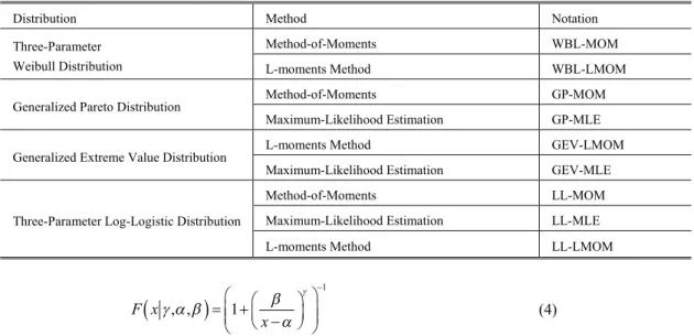
In order to estimate the maximum pressure, 4 statistical models are applied, which are three-parameter Weibull distribution (WBL), generalized Pareto distribution (GP), generalized extreme value distribution (GEV) and three-parameter log-logistic distribution (LL). The cumulative distributions of statistical models are given below.

Three-parameter Weibull distribution (WBL)

(

)

Generalized Pareto distribution (GP)

(

)

Generalized extreme value distribution (GEV)

(

)

(

)

Table 1. Parameter estimation method for distribution and notation for each fit

Distribution Method Notation

Three-Parameter Weibull Distribution

Method-of-Moments WBL-MOM

L-moments Method WBL-LMOM

Generalized Pareto Distribution Method-of-Moments GP-MOM

Maximum-Likelihood Estimation GP-MLE

Generalized Extreme Value Distribution L-moments Method GEV-LMOM Maximum-Likelihood Estimation GEV-MLE

Three-Parameter Log-Logistic Distribution

Method-of-Moments LL-MOM

Maximum-Likelihood Estimation LL-MLE

L-moments Method LL-LMOM

(

)

Where γ is the shape parameter, α is the location parameter and β is the scale parameter and variable x should be equal or larger than the location parameter. In case of generalized Pareto distribution, Peak-Over-Threshold (POT) method is applied for better fitting. In POT method, only the data exceeds a certain threshold value is taken into consideration. In this study, the 0.92 quantile of the sample peaks is consid-ered as the threshold value which means 8% largest peaks are considconsid-ered for generalized Pareto distribu-tion. The three-parameter log-logistic distribution is often used in estimating flood frequencies in hydrolo-gy, but has never been to sloshing peak pressures yet.

2.2. Distribution Fitting Methods

In the distribution fitting process, it is very important to find an appropriate method for estimating. Differ-ences in these parameters can change the shape of the fitting and cause a large difference in the prediction of maximum pressure. In this study, three methods were used to estimate the parameters suitable for vari-ous statistical models, which are maximum likelihood estimation (MLE), method-of-moments (MOM), and l-moment method (LMOM).

MLE is a method developed by R.A. Fisher in the 1920’s to find the probability distribution that makes the obtained data most probable by maximizing the likelihood function. If sample size is small, MLE can give biased estimation. For WBL, MLE can be applied under limited conditions where shape factor is greater than 1, but in the case of peak pressure, shape parameter is usually smaller than one. Therefore, MLE is not suitable to use for WBL.

MOM is a method of estimating parameters by matching three model moments –mean, variance, and skewness- with their corresponding sample moments. MOM has a limitation that the moments more than the second order must be defined in a certain range of the shape parameter. In case of GEV, the mean and variance are infinite when the shape parameter is greater than 1 and 1/2, respectively. Since the parameter estimation is not possible within the specific range of shape parameter, the MOM method has not been applied to GEV in this study.

LMOM is method described by Hosking(1990), and an alternative approach to MOM. L-moments are similar to conventional moments, but can be estimated as a linear combination of order statistics. LMOM matches L-moments and L-moments ratios of the distribution with their corresponding sample L-moments and L-moment ratios.

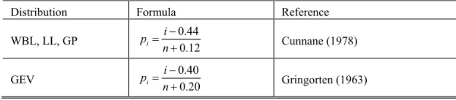
Table 2. Plotting position formulas

Distribution Formula Reference

WBL, LL, GP 0.44 0.12 i i p n -= + Cunnane (1978) GEV 0.40 0.20 i i p n -= + Gringorten (1963) 2.3. Goodness-of-Fit Test

Probability plot correlation coefficient (PPCC) test is used to examine the goodness-of-fit. PPCC test was first proposed by Filiben(1975) and later developed to be applicable for other distributions as well as nor-mal distribution. The r used in this test is a coefficient indicating the relationship between the ordered servations Xi and fitted quantiles Mi determined by plotting positions pi for each Xi. Assume that the ob-servations can be derived from the fitted distribution when the value of r is close to 1.0. Fundamentally, r provides a quantitative evaluation of fitness by measuring the linearity of the probability plot (Heo at al., 2008). The correlation coefficient r is defined as below.

(

)(

)

(

) (

)

-å

å

å

X and M denote the mean values of the observations Xi and the fitted quantiles Mi, respectively and n is

the sample size. The estimate of order statistic median for Mi is shown as,

1

( )

( )

( )

Φ-1 is the inverse of cumulative distribution function. Equation (10) is the plotting position formula of normal distribution. Plotting position formulas used for other distributions are shown in Table 2.

For hypothesis testing, critical values are obtained by Monte-Carlo simulations. 105 random samples such as the sample size of the peak pressure data are generated from fitted distributions and PPCC test is per-formed for each random samples. Significance level is set at 0.05. Therefore (105×(1-0.05))th highest PPCC is chosen as the critical value (Vogel, 1986). If the PPCC of the pressure data is higher than the criti-cal value, then hypothesis return 0, otherwise returns 1. A return value of 0 means that at the set significant level, the data is extracted from the distribution.

3. Sloshing Experiment

The experiments were carried out at Seoul National University (SNU) sloshing experiment facility. There are three hexapod motion platforms with different payloads (1.5, 5, and 10ton) in SNU. In this study, 5-ton

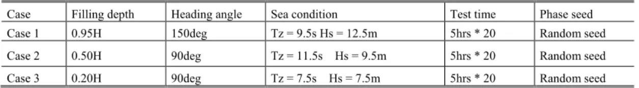
Table 3. Test conditions

Case Filling depth Heading angle Sea condition Test time Phase seed

Case 1 0.95H 150deg Tz = 9.5s Hs = 12.5m 5hrs * 20 Random seed

Case 2 0.50H 90deg Tz = 11.5s Hs = 9.5m 5hrs * 20 Random seed

Case 3 0.20H 90deg Tz = 7.5s Hs = 7.5m 5hrs * 20 Random seed

Table 4. Selected four panels according to load condition

0.20H 0.50H 0.95H Panel NO. 14 4 1 19 6 2 22 14 4 23 16 6

payload hexapod motion platform was used with a tank whose length (L) is 868.2 mm, width (B) is 760 mm, and height (H) is 555mm. In the extreme wave condition, 5-hour-test based on real scale was scaled down with Froude scaling and carried out 20 times. Test conditions are shown in Table 3. The experiment was carried out at three different loading conditions: 0.20H, 0.50H, 0.95H with different heading angle and sea condition.

The tank is based on 140K Liquefied Natural Gas Carrier (LNGC) with a 1:50 scale ratio. In order to avoid the effect of hydroelastic response of tank, tank is made by plexiglass whose thickness is 35-40 mm. Integrated circuit piezoelectric (ICP) sensors were mounted as cluster panels to measure the dynamic pres-sure on the tank. The layout of panels is shown in Fig. 2.

Fig. 1 Experiment setup Fig. 2 Layout of sensor cluster panels

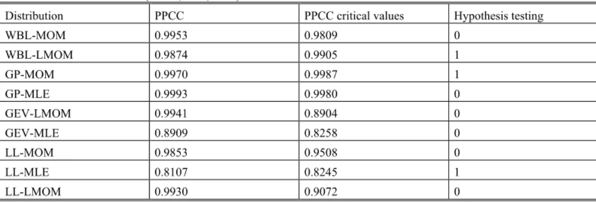
Table 5. PPCC test results of (0.20H, P.19, No.5)

Distribution PPCC PPCC critical values Hypothesis testing

WBL-MOM 0.9953 0.9809 0 WBL-LMOM 0.9874 0.9905 1 GP-MOM 0.9970 0.9987 1 GP-MLE 0.9993 0.9980 0 GEV-LMOM 0.9941 0.8904 0 GEV-MLE 0.8909 0.8258 0 LL-MOM 0.9853 0.9508 0 LL-MLE 0.8107 0.8245 1 LL-LMOM 0.9930 0.9072 0

Once the pressure data is measured, low-frequency (lower than 50HZ) drift is removed through a high-pass filter. In order to statistically analyze the sloshing load, impact pressure is identified using peak-over-threshold (POT) method. The peak-over-threshold value set in the experiment is 2.5 kPa, and the size of sampling time window for the peak pressure value detection is 0.2 sec (Kim et al., 2014). Four panels with high im-pact pressures were selected for each loading condition, and statistical analysis was performed based on the peak pressure measured on the four selected panels (Table 4).

4. Results

4.1. Short Duration Test

The parameter estimates for each distribution are based on the peak pressure data obtained from the four panels at each loading condition. For statistical analysis, probability of exceedance curves are obtained for each fit and the PPCC tests are performed. The results obtained from panel 19 of the fifth test with a filling level of 0.20H were statistically analyzed and shown in Fig. 3 and Table 5. For convenience, the above conditions are expressed in the following notation (0.20H, P.19, No.5), and the notation will be used here-after when referring to the data. Normalized pressure value which is in x-axes, is calculated as P/ρgH where P is the magnitude of pressure, ρ is the density, g is the gravity and H is the height of the tank

(a) 0.50H, P.14, No.13 (b) 0.95H, P06, No.15

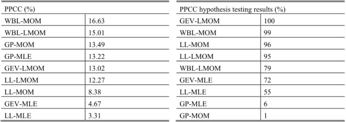
Table 6. PPCC test results for whole data

PPCC (%) PPCC hypothesis testing results (%)

WBL-MOM 16.63 GEV-LMOM 100 WBL-LMOM 15.01 WBL-MOM 99 GP-MOM 13.49 LL-MOM 96 GP-MLE 13.22 LL-LMOM 95 GEV-LMOM 13.02 WBL-LMOM 79 LL-LMOM 12.27 GEV-MLE 72 LL-MOM 8.38 LL-MLE 55 GEV-MLE 4.67 GP-MLE 6 LL-MLE 3.31 GP-MOM 1

GEV-MLE and LL-MLE apparently did not fit well and PPCC values were also low. For other distribu-tions, it is seen that POE curves and PPCC values are in accordance. In the case of GEV-MLE, the PPCC value is low, but the PPCC critical value was lower, so the hypothesis test result was not rejected. There-fore, it is difficult to apply the hypothesis method as reference in the comparison of the fits.

The POE curves at different test condition are shown in Fig. 4. These figures show the representative cas-es where high impact prcas-essurcas-es occur at each filling level. The thrcas-eshold used in GP is shown in the figure for easy identification. As in the above conditions, GEV-MLE and LL-MLE cases show the worst fit in the figure.

The PPCC values for each distribution are compared for all test conditions. Based on the PPCC results of each distribution, the ranking is averaged over 20 repeated tests and the ratios of the ranks are shown in Table 6 as percentages. In the case of hypothesis test, the acceptance ratios of each fits are also summarized in Table 6. According to the PPCC test results for the whole data set, WBL has the highest goodness-of-fit rate, followed by GP. For these two statistical models, MOM gives a better fit than L-MOM. As expected from the figures, GEV-MLE and LL-MLE fits are rated lowest.

There are some aspects to consider when comparing fittings based on the whole data set. PPCC test is a method sensitive to the size of the sample. In the lower tail of a distribution with smaller values, a large amount of data is gathered, but in an upper tail containing higher values, the number of data is small.

(a) 0.50H, P.04, No.04 (b) 0.20, P.22, No.19

Table 7. PPCC test results of tail-only data PPCC - tail 0.20H (%) PPCC - tail 0.50H (%) WBL-MOM 15.1 WBL-MOM 14.9 GP-MLE 15.1 WBL-LMOM 13.4 LL-MOM 14.7 LL-MOM 13.2 GP-MOM 13.9 GP-MOM 12.5 LL-LMOM 12.3 LL-LMOM 12.0 GEV-LMOM 10.8 GP-MLE 11.8 WBL-LMOM 10.7 GEV-LMOM 11.5 GEV-MLE 4.9 GEV-MLE 5.7 LL-MLE 2.6 LL-MLE 5.0

PPCC - tail 0.95H PPCC – tail total

WBL-MOM 16.1 WBL-MOM 15.4 LL-MOM 14.7 LL-MOM 14.2 WBL-LMOM 13.8 GP-MOM 13.2 GP-MOM 13.2 GP-MLE 13.2 GP-MLE 12.9 WBL-LMOM 12.7 LL-LMOM 12.1 LL-LMOM 12.1 GEV-LMOM 9.5 GEV-LMOM 10.6 LL-MLE 4.2 GEV-MLE 4.7 GEV-MLE 3.5 LL-MLE 3.9

Therefore, a larger sample size in the distribution has a greater impact on the PPCC value. In this case, the lower values of distribution are perfectly fitted but the higher values provide poor fit from the upper tail. Unlike other distributions that use whole data set, a comparison with GP using only the peak value of the upper 8% may be a problem. This is because the parameters are obtained by using the peak data of the up-per 8% and then expanded to the distribution of the whole data set with the same parameter. Therefore as shown in Fig. 5, the fit of GP is good in the higher impact pressure region, but the fit may appear to be poor in the whole data.

The hypothesis testing results show that even though PPCC rate of GP is high, the acceptance rate is low-er than 10%. If the data has extreme values near the upplow-er tail or if the shape of data changes significantly in the upper tail, GP fit does not follow the shape of whole data. This is the reason why hypothesis ac-ceptance rate of GP is low. It is questionable to compare the goodness-of-fit test of whole data, since the distribution of the upper tail side, including the high impact pressure values, is more important from a de-sign standpoint.

Table 8. PPCC test result for 100 hours of whole data and tail-only data

PPCC 100 hours PPCC tail 100 hours

GP-MOM 22.22 WBL-MOM 21.83 GP-MLE 21.83 GP-MOM 20.63 WBL-MOM 19.05 GP-MLE 19.44 WBL-LMOM 15.48 LL-MOM 17.06 LL-LMOM 11.11 WBL-LMOM 11.90 LL-MOM 10.32 LL-LMOM 9.13

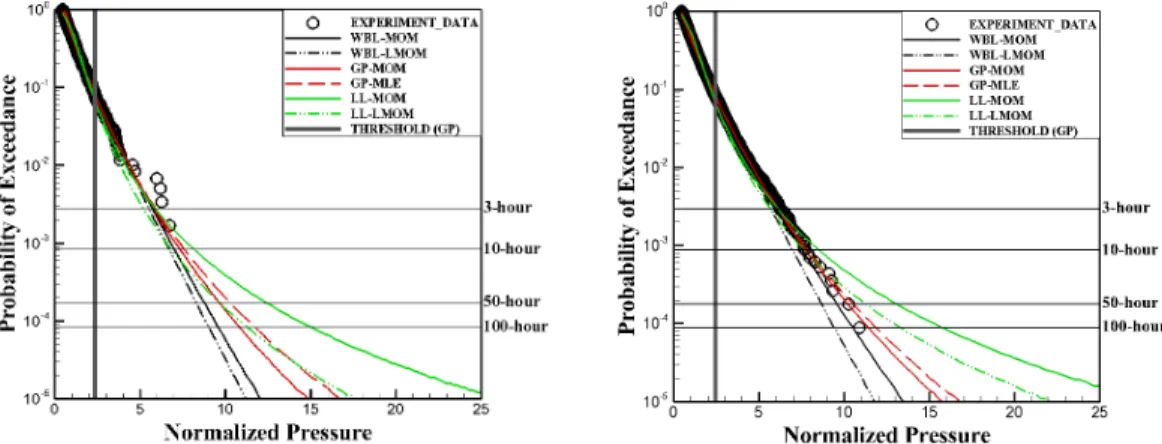
Fig. 6 POE curves of 5-hour experiment(left, 0.20H, P.14, No.09) and 100-hour experiment(right)

In order to overcome the problem in the goodness-of-fit evaluation, PPCC test was applied with samples whose peak pressures are larger than threshold of 0.92 quantile. PPCC tail-only results for each filling level, and for all conditions are shown in percent in Table 7. WBL-MOM gave the best fit in the tail for compre-hensive conditions followed by LL-MOM. GP fits occupied the third and fourth place, but was slightly different from WBL-MOM and LL-MOM. According to PPCC tail-only results, MOM gave a better fit than LMOM method, and MLE showed the poorest fit in this study, especially for distributions with three parameters.

4.2. Long Duration Test

The object of this study is to find the best fit to estimate the maximum pressure and compare the distribu-tion results for the long duradistribu-tion as well as the short duradistribu-tion. To find this, the results of distribudistribu-tion by short duration as well as distribution by long duration were also compared. Based on the results of previous comparisons, the GEV-MLE, GEV-LMOM, and LL-MLE fits which estimated exaggerated maximum pressure were excluded in long duration comparisons. The 100-hour experimental results were obtained by rearranging the peak pressures after integrating all of the 20 repeated 5-hour experiments. The PPCC result for whole data and the tail-only data for comprehensive conditions are shown in Table 8. GP showed the best fit regardless of the parameter estimation method for whole data, and WBL-MOM showed the best fit for tail-only data in long duration data. The top three methods are now widely used, and the difference in results is not large.

The POE curves of the 5-hour experimental result and the 100-hour experimental result are shown in Fig. 6, and the straight lines corresponding to the return period of 3, 10, 50, 100 hours are also shown. The re-sults of the 100-hour experiment show higher convergence than the 5-hour experiment, and it ca be con-firmed that the higher impact pressure can be more accurately predicted. As the return period becomes longer, the pressure estimation value increases in the order of WBL, GP, and LL. While the LL curve shows the overestimated values, the GP curve is similar to the experimental results. Among the three pa-rameter estimation methods, MOM provides an estimation curve that is the closest to the experimental re-sult.

5. Conclusion

Three-parameter Weibull, generalized Pareto, generalized extreme value and three parameter log-logistic distributions are fitted to peak pressure measure from 20 repeated 5-hour experiments using three different parameter estimation methods. The goodness-of-fit is compared for each fitting by PPCC test and observa-tions of probability of exceedance curves.

It is difficult to fit with the maximum likelihood estimation method for distribution with three parameters. Among the other two parameter estimation method, the more suitable method for this study was moment-of-method than L-moment method.

Although the three-parameter log-logistic distribution showed good fit in short duration, it showed exag-gerated results from long duration to long-term prediction. Generalized extreme value distribution also showed the overestimated pressure values, so these two distributions are not suitable for peak pressure modeling.

Three-parameter Weibull model using method-of-moments showed the highest goodness-of-fit test results in the tail for both short duration and long duration. Generalized Pareto distribution is also suitable to mod-el for peak pressure since it showed the best fit among the long-duration test for whole data set.

Acknowledgements

This study has been studied as a part of PRESLO JIP which had been supported by ABS, ClassNK, DSME, HHI, KR, LR, SHI, STX. Also, some studies were supported by the Lloyd’s Register Foundation (LRF)-Funded Research Center at Seoul National University. The support of all sponsors is greatly appre-ciated.

References

Cousineau, D., “Nearly Unbiased Estimators For the Three Parameter Weibull Distribution With Greater Efficiency Than the Iterative Likelihood Method,” Brit J Math Stat Psychology, 62, 167-191, 2009. Cunnane, C., “Unbiased Plotting Positions – A Review,” J Hydrology, 37(3/4), 205-222, 1978.

Filliben, JJ (1975). “The Probability Plot Correlation Coefficient Test For Normality,” Technometrics, 17(1), 111-117.

Fillon, B, Diebold, L, Henry, J, et al., “Statistical Post-Processing of Long-Duration Sloshing Test,” Proc 21th Int Offshore and Polar Eng Conf, Hawaii, ISOPE, 46-53, 2011.

Grazcyk, M, Moan, T and Rognebakke, O., “Probabilistic Analysis of Characteristic Pressure for LNG Tanks,” J Offshore Mech Arct, 128, 133-134, 2006.

Grazcyk, M and Moan, T., “A Probabilistic Assessment of Design Sloshing Pressure Time Histories in LNG Tanks,” Ocean Eng, 35, 834-855, 2008.

Gran, S., “Statistical Distributions of Local Impact Pressures,” Norweg Marit Res, 8(2), 2-13, 1981. Gringorten, II., “A Plotting Rule for Extreme Probability Paper,” J Geophysical Res, 68(3), 813-814, 1963. Heo, J-H, Kho, YW, Shin, H, Kim, S., “Regression Equations of Probability Plot Coefficenttest Statistics

From Several Probability Distributions,” J Hydrology, 355, 1-15, 2008.

Hosking, JRM., “L-Moments: Analysis and Estimation of Distributions Using Linear Combinations of Order Statistics,” J Royal Stat Society Series (B) Method, 52(1), 105-124, 1990.

Kim, SY, Kim, Y, Kim, KH., “Statistical Analysis of Sloshing-Induced Random Impact Pressures,” Proc Inst Mech Eng, Part M: J Eng Maritime Environ, 228(3), 235-248, 2014.

Kuo, JF, Campbell, RB, Ding, Z, et al., “LNG Tank Sloshing Assessment Methodology – The New Gener-ation,” Int J Offshore and Polar Eng, ISOPE, 19(4), 241-253, 2009.

Mathiesen, J., “Sloshing Loads Due to Random Pitching,” Norweg Marit Res, 3(2), 2-13, 1976. Myung, IJ., “Tutorial on Maximum Likelihood Estimation,” J Math Psychology, 47, 90-100, 2003. Pickands, J III., “Statistical Inference Using Extreme Order Statistics,” Ann Stat, 3(1), 119-131, 1975. Smith, RL., “Maximum Likelihood Estimation In A Class Of Nonregular Cases,” Biometrika, 72, 67-90,

1985.

Vogel, RM., “The Probability Plot Correlation Coefficient Test for Normal, Lognormal, and Gumbel Dis-tributional Hypotheses,” Water Resources Res, 22(4), 587-590, 1986.