Quarterly livestock model

(1)

QUARTERLY

LIVESTOCK MODEL

Korea Rural Economic Institute

Food and Agricultural Policy Research Institute

(2)

(3)

(4)

SUMMARY

The review of each Korean livestock sector provided the background needed to develop an econometric version of the sectors. The first step in the process was the estimation of each of the identified behavioral equations. Chapter 3 provides the results of the estimations. Each equation has an identified R-square, Durbin-Watson statistic and a t-statistic for each parameter in the equation. A variable definition list can be found near the end of chapter 3.

The general approach used in each sector was to first identify the primary supply point. In the case of beef it is the number of female cows greater than two years of age. For pork, it is the number of sows in the pork herd while for chickens the number of chickens hatched drives the supply side.

Each of these equations has a similar specification. These equations contain a lagged dependent variable to help capture the dynamics of the supply portions of the sectors. A ratio of output to input prices is also contained in the equations that drive the response of these equations to changing economics. The reader can look in the equations sheet of the Excel model to find the short and long run elasticities of each of the equations.

At the other end of the spectrum, each of these sectors contains primary domestic consumption equations. The consumption of each meat product depends on its own price, the price of the other two meats in the system and income. Since these equations are estimated in double-logarithmic form the coefficients can be interpreted as elasticities. The demand side of this model remains estimated in a single equation approach rather than using a system approach as the lack of precision in gathering the data causes a system approach difficulties even though it allows for more demand theory to be imposed on the system.

The other important portion of the model is the interaction with world markets. Trade equations are estimated that include comparisons of world to domestic prices, exchange rates and other trade barriers that limit trade to something less than the free trade solution.

A beef import and chicken net trade equations are estimated in the system. No trade equations are estimated for pork since trade has been a very small portion of the Korean pork market.

The remaining equations provide two primary functions to the model. First, the remaining supply equations ensure that the biological constraints of each of the sectors are not violated. That is, animals or meat are not created or lost in the system. These equations will ensure that when a calf, pig or chick is born that the

(5)

animal remains in the system until it is slaughtered, dies or goes back to the breeding herd.

The other set of equations provide the means of translating retail meat prices back to producers. Many of these equations can be classified as derived demand equations that show what an actor is willing to pay for an animal of a particular size and age to turn it into the next stage of the process. The most obvious case is what a meat processor is willing to pay for live animals to turn them into meat.

Although estimation of each of these behavioral equations is important in building the model, the larger objective is to have a system that performs satisfactorily. Tables on the first two pages of appendix 2 provide performance statistics of the entire system over the 1995 to 2002 period. These statistics are dynamic in that errors in one year are allowed to be carried into subsequent years. The far right column of these tables provides the annual percent root mean square error for all endogenous variables. In general, the beef model performs the most poorly of the sectors but that is expected given the number of lags that are contained in the model. Even though it performs the least satisfactorily, many of the errors are below 20 percent. The pork and chicken sectors perform very well over the period. Appendix 2 provides graphics of the actual versus predicted values from the dynamic simulation.

(6)

Tables

Table 1. Korean Livestock Industry in the Agricultural Sector ……… 1

Table 2. Korean Beef Supply and Utilization ……… 4

Table 3. Cattle Procurement by Local Cattle Market ……… 5

Table 4. Cattle Slaughter Rate by Slaughter Plants, 2001.12 ……… 6

Table 5. Korean Pork Supply and Utilization ……… 8

Table 6. Korean Chicken Supply and Utilization ……… 10

Figures

Figure1. Korean Beef Flow Diagram ……… 3

Figure 2. Korean Beef Cattle and Korean Beef Marketing Process Local Cattle Market 5 Figure 3. Hog, Retail pork, and Farm-Retail price spreads ……… 9

(8)

1. INTODUCTION

In July 2004 the Food and Agricultural Policy Research Institute (FAPRI) at the University of Missouri and the Korean Rural Economic Institute (KREI) entered into an agreement that would result in a quarterly Korean livestock model to be estimated by FAPRI. The beef, pork and chicken sectors are modeled in this project. The model is econometrically estimated and produced in an Excel spreadsheet.

The steps followed in constructing the model are: 1) a review of the Korean livestock industry, 2) theoretical development of the model, 3) single equation estimation of the behavioral equations and 4) simulation of the simultaneous system of equations. This paper will provide a summary of this process to provide insight into the final model delivered to KREI. In addition, appendices are added that summarize a procedure of using the Excel model.

2. REVIEW OF THE KOREAN LIVESTOCK INDUSTRY

Livestock industry in Korea has continuously grown and gains an importance in the entire agricultural sector. The gross value of livestock production rose from about 6000 billion won in 1995 to about 9,000 billion won in 2003 (Table 1). Livestock production accounted for 23 percent of total agricultural products in 1995 and rose to 28 percent of total agricultural products in 2003 (Table 1).

Table 1. Korean Livestock Industry in the Agricultural Sector

1995 1998 1999 2000 2001 2002 2003

(Billion Won)

Livestock Production (A) 5958 7515 7937 8082 8312 9052 8869

Cattle (B) 1776 1836 1778 1878 1700 2136 2463

Swine (C) 1406 2390 2687 2372 2692 2918 2681

Broiler (D) 773 858 768 821 863 729 641

Agriculture (E) 25855 29638 31857 31828 32447 32147 31809

(Percentage)

Livestock Share in Agriculture (A/E) 23.0 25.4 24.9 25.4 25.6 28.2 27.9 Cattle Share in Livestock (B/A) 29.8 24.4 22.4 23.2 20.5 23.6 27.8 Swine Share in Livestock (C/A) 23.6 31.8 33.9 29.3 32.4 32.2 30.2 Broiler Share in Livestock (D/A) 13.0 11.4 9.7 10.2 10.4 8.1 7.2 Source: MAF, Statistical Yearbook of Agricultural and Forestry, 2004.

(9)

2.1. BEEF

2.1.1. BEEF INDUSTRY SITUATION

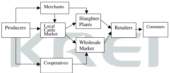
The Korean beef flow diagram in Figure 1 describes the underlying structure and price determination process of Korean beef cattle industry. This diagram shows the flow of product through the market channel from the cow-calf producer to the consumer of the beef product.

Beef cattle farms in Korea are specialized by cow-calf producers and cattle feeders. The majority of cow-calf producers are smaller volume farms which have less than 30 head of cattle and calves. Cattle feeders are rather larger volume operations which have over 30 head of cattle. Cow-calf producers having 20-30 head of cattle and calves change their business type to cattle feeder if relative income in feeding cattle is expected to increase.

The number of beef cattle farms has continued to decrease. Between 1990 and 2003, the number of beef cattle farms has decreased from 620 thousand to 188 thousand households (Table 2). The majority of beef cattle farms are still small scale farms having less than 50 heads of cattle but the proportion of large scale farms in the number of beef cattle has continued to grow. In 1990 the beef cattle farms having less than 50 head accounted for 99 percent of total beef cattle farms and the proportion of beef cattle on farms having less than 50 head accounted for 95 percent of total beef cattle. In 2003 the proportion of beef cattle on farms having less than 50 head accounted for only 67 percent of total beef cattle (Table 2).

The number of beef cattle on farms has increased until late 1997. However, the beef cattle industry had undergone severe contraction from late 1997 to early 2001 because of a financial crisis in late 1997. The high imported feed grain prices attributable to high exchange rate by the financial crisis in late 1997 deteriorated the profitability of beef cattle farms and forced them to slaughter breeding cows. For example, the number of female beef cattle slaughtered rose from 92 thousand heads in second quarter of 1997 to 166.7 thousand heads in third quarter of 1997-81 percent increase from a previous quarter. Increasing number of slaughtered animals decreased farm price of fed steers (i.e. 500 kg male beef cattle) and in turn decreased calf price. Beef cow over 2 years old decreased from 1.2 million heads in second quarter of 1997 to 525 thousand heads in second quarter of 2002. Beef cattle breeding herd slowly expanded since early 2002.

A growing insecurity of beef producers about trade liberalization as a result of the Uruguay Round agricultural agreement, Korean beef production decreased from 264 thousand ton in 1998 to 142 thousand ton in 2003- 46 percent decrease (Table 2). Decreasing domestic production was balanced by increasing imports to

(10)

meet sustaining beef consumption. Beef imports increased from 77 thousand ton to 294 thousand ton during the same period- 282 percent increase (table 2). However, a beef imports in 2004 is projected to fall by almost 50 percent from a previous year due to a BSE (Bovine Spongiform Encephalopathy) outbreak in U.S.A. The majority of imported beef is from the U.S.A. and Australia. U.S.A. accounted for 68 percent of total beef imports in 2003 (Jeong, P.14).

Figure1. Korean Beef Flow Diagram1

1

Huh, Duk. et al., Outlook and Policy for Korean Beef Industry. KREI. 2001. P.25.

Production cost of calf > Calf price = Number of Calves decrease

Production cost of calf < Calf price = Number of Calves increase

Cattle and calves on farm Cow-calf farms

Cattle feeding

farms Calf price Calf supply < calf demand =Price increase Calf supply > calf demand = Price decrease

Growing cost of feeder cattle

Fed cattle price Cattle on

feed

Fed cattle price > Growing cost of feeder cattle = cattle on feed decrease

Fed cattle price < Growing cost of feeder cattle = cattle on feed decrease

Cattle placed in the market

Cattle and calves on farm

Wholesale price Cattle placed in the market <Wholesaler demand = wholesale price increase Cattle placed in the market > Wholesaler demand = wholesale price decrease. Korean Beef

(Hanwoo) demand Per capita

income Korean beef price

(11)

Table 2. Korean Beef Supply and Utilization 1990 1996 1997 1998 1999 2000 2001 2002 2003 (1000 Household) Number of Household 1-19 Head 615 489 439 404 331 274 221 197 172 20-49 Head 4.5 22 22 18 15 11.3 10.6 10.8 11.4 50-99 Head 0.8 2.3 3.2 3.9 3.5 2.9 2.8 2.9 3.7 Over 100 Head 0.2 0.5 0.9 1.1 1.2 1.1 1.1 1.3 1.4 Total 620 513 464 427 350 289 235 212 188 (1000 Head) Number of Beef Cattle On Farms having 1-19 Head 1402 1996 1739 1404 1063 858 693 656 650 20-49 Head 131 607 639 532 440 334 314 320 341 50-99 Head 51 145 201 254 233 194 186 192 236 Over 100 Head 37 96 157 193 216 204 212 242 254 Total 1622 2844 2735 2383 1952 1590 1406 1410 1480 (1000 Tons) Supply Beginning Stocks 4 6 4 47 42 39 73 18 55 Imports 82 147 168 77 163 223 166 292 294 Production 95 174 237 264 227 214 163 147 142 Total 181 327 409 388 432 476 402 458 490 Utilization Consumption 177 323 362 345 393 402 384 403 390 Exports 0 0 0 0 0 0 0 0 0 Ending stocks 4 4 47 42 39 73 18 55 100 Total 181 327 409 388 432 476 402 458 490 (Kilograms) Per Capita Consumption Retail Weight 4.13 7.14 7.93 7.44 8.38 8.51 8.05 8.50 8.14 Prices (1000 Won / 500Kg) Female Beef Cattle 2147 2853 2159 1887 2410 2872 3514 4236 4849

Male Beef Cattle 2405 2848 2426 2007 2488 2752 3245 3927 3907

(1000 Won / Head) Female Calf 867 1506 733 535 774 1103 1729 2306 3242

Male Calf 1217 1567 1046 658 1024 1294 1785 2288 2610

(Won / 500g) Retail Beef 5658 8118 7537 6911 7235 8709 9617 14739 15650

Source: NACF, Materials on Price, Supply & Demand of livestock Products, 2004. NAQS, Livestock Statistics, 2004.

(12)

Producers Merchants Local Cattle Market Wholesale Market Retailers Cooperatives Consumers

2.1.2. BEEF MARKETING CHANNELS

Korean beef cattle are purchased through merchants connected to retailers, local cattle markets, or local livestock cooperatives (Figure 2). A majority of the procured cattle by merchants are slaughtered by private slaughter plants and then directly marketed to retailers. Procured cattle through cooperatives are slaughtered at the wholesale market and the carcass prices are set by auction.

Figure 2. Korean Beef Cattle and Korean Beef Marketing Process Local Cattle Market2

Slaughter Plants

2.1.3. LOCAL CATTLE MARKET

The number of cattle placed in the local cattle market decreased from 1,257 thousand head in 1990 to 515 thousand head in 2001. In the same period, the number of local cattle market reduced from 287 to 106 markets because of mergers and closures of small scale markets (Table 3).

Table 3. Cattle Procurement by Local Cattle Market

1990 2001

Number of local cattle Markets 287 106

Cattle placed (1000 head) 1,251 515

Cattle marketed (1000 head) 951 345

Rate of marketed (%) 76.0 67.1

Source: Jeong, M.K. et al., An Analysis on Beef Marketing and Consumption pattern, KREI, 2002. P.14.

2

(13)

2.1.4. SLAUGHTER PLANTS

Slaughter plants in Korea are characterized as a small scale operation, low average daily slaughter rate, and low-profitability. The number of slaughter plants reduced from 179 in 1980 to 113 in 2001 and average daily slaughter rates for cattle and hogs in 2001 were, respectively, 23.2 percent and 45.7 percent of physical capacity of slaughter plants (Table 4).

The Government established LPC (Livestock Processing Complex) which slaughters animals, fabricates meats, and sells carcass in one place started in 1994. In slaughter capacity, LPC accounted for 7 percent of cattle marketed and 13.3 percent of hogs marketed in December 2001. In average daily slaughter rate, LPC accounted for 6.1 percent of cattle marketed and 11 percent of hogs marketed in December 2001.

Table 4. Cattle Slaughter Rate by Slaughter Plants, 2001.12

Slaughter Capacity (Head/ Day) Actual Slaughter (Head/ Day) Slaughter Rate (%) Number

Cattle Hogs Cattle Hogs Cattle Hogs

Private 102 9,209 (87.2) 92,659 (88.1) 1,909 (78) 37,985 (79.1) 20.7 41.0 State 4 118 (1.1) 361 (0.3) 17 (0.7) 66 (0.1) 14.4 18.3 Cooperatives 7 1,232 (11.7) 12,148 (11.6) 521 (21.3) 10,017 (20.8) 42.3 82.5 Total 113 10,599 (100) 105,168 (100) 2,447 (100) 48,068 (100) 23.2 45.7

Source: Jeong, M.K. et al., An Analysis on Beef Marketing and Consumption pattern, KREI, 2002. P.15.

2.1.5. RETAILERS

Beef is purchased by local butchers, supermarkets, and restaurants, etc. Local butchers account for 65.3 percent from total beef retailers. Imported beef has seen a continual increase. Imported beef was only sold at the retailers that

specialized in imported beef until 2001. WTO banned separating Korean beef retailers and imported beef retailers and forced to sell both Korean beef and imported beef together since 2001.

(14)

2.2. PORK

2.1.1. PORK INDUSTY SITUATION

The swine industry has increased continuously and continues to gain importance in the entire meat complex. Total product value of swine industry in 2003 was 2681 billon won and it was the highest in the entire meat complex (Table 1).

Hog farms are continuing to become larger. The number of hogs on farm has continued to rise while the number of hog farms has decreased continuously. Between 1990 and 2003, the number of hogs on farms has increased from 4.5 million to 9.2 million heads while the number of hog farms has decreased from 133 thousand to 15 thousand households (Table 5). During the same period, the proportion of hog farms having more than 1000 head has rose from 0.3 percent to 22 percent of total hog farms and the proportion of hogs on farms having more than 1000 head has rose from 23 percent to 75 percent of total hogs on farm (Table 5).

There are 87 swine growing complexes and 17 packers who vertically coordinate hog production operations in March 2001 (MAF, 2001). Hogs involved with swine growing complexes or vertically coordinated operations accounted for 52 percent of total hogs on farms in March 2001. Majority of hog farms having more than 500 heads either horizontally coordinated with swine growing complexes or vertically coordinated with packers (MAF, 2001).

Pork production has increased from 507 thousand ton in 1990 to 783 thousand ton in 2003. During the same period, pork consumption has increased from 505 thousand ton to 834 thousand ton in 2003 (Table 5). Pork consumption accounted for largest proportion of entire meat consumptions. Per capita pork consumption in 2003 was 17.4 kg and accounted for 52 percent of per capita meat consumption.

Pork imports have risen from 3 thousand ton in 1990 to 61 thousand ton in 2003. During the same period, pork exports have risen 6 thousand ton to 27 thousand ton (Table 5). Pork exports had increased sharply from 1997 to 1999 as a result of an increase in exports to Japan but pork exports were sharply curtailed in 2000 due to a breakout of FMD (Foot and Mouse Disease) in Korea and have slowly recovered the last few years.

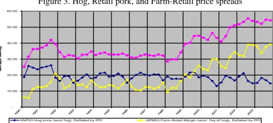
Deflated live hog prices per kilogram were quite volatile while deflated retail pork prices per 560 gram were relatively constant over the over 1991/1-1996/12 periods. In addition to farm and retail price changes, live hog prices and farm-retail hog price spreads had negative correlation over the same period; farm-retail price spreads increase (decrease) when farm level live hog prices decrease (increase).

(15)

Kim (1998) argued that this monthly prices and price spread movements stem from exploitation of market power by pork retailers. This asymmetric movement between farm-retail hog price spreads and farm level live hog prices have sustained until 2003 (Figure 2).

Table 5. Korean Pork Supply and Utilization

1990 1996 1997 1998 1999 2000 2001 2002 2003 (1000 Household) Number of Household 1-999 Head 133 32 25 25 22 22 17 14 12 1000-4999 Head 0.4 1.2 1.6 1.8 2.0 2.2 2.6 2.8 2.7 5000-9999 Head 0.03 0.04 0.06 0.06 0.06 0.09 0.1 0.1 0.1 Over 10000 Head 0.01 0.02 0.03 0.03 0.04 0.04 0.04 0.05 0.05 Total 133 33 27 27 24 24 20 17 15 (1000 Head) Number of Hogs On Farms having 1-999 Head 3475 3734 3584 3636 3419 3271 2890 2525 2197 1000-4999 Head 703 2080 2638 3100 3529 3820 4512 4902 5057 5000-9999 Head 196 292 423 437 435 629 690 807 871 Over 10000 Head 153 410 450 371 480 494 628 675 777 Total 4528 6516 7096 7544 7864 8214 8720 8974 9231 (1000 Tons) Supply Beginning Stocks 2 4 4 18 17 25 39 30 58 Imports 3 41 65 56 142 96 102 71 61 Production 507 692 699 733 701 714 733 785 783 Total 511 738 767 806 861 835 875 886 901 Utilization Consumption 505 697 698 701 755 780 807 810 834 Exports 6 37 52 88 80 16 38 18 27 Ending stocks 0 4 18 17 25 39 30 58 40 Total 511 738 768 806 861 835 875 886 901 (Kilograms) Per Capita Consumption

Retail Weight 11.7 15.4 15.3 15.1 16.1 16.5 16.8 17.0 17.4 Prices (1000 Won / 100Kg) Hog (100Kg) 164 171 171 179 199 166 174 178 164 (Won / 500g) Retail Pork 2125 2447 2554 2805 3723 3883 4224 4769 4849

(16)

Figure 3. Hog, Retail pork, and Farm-Retail price spreads -10.00 20.00 30.00 40.00 50.00 60.00 199 0 199 1 199 2 199 3 199 4 199 5 199 6 199 7 199 8 199 9 200 0 200 1 200 2 200 3 w on/ k g o f l iv e ho g

ANP53 Hog price (won/1kg), Deflated by PPI APM53 Farm-Retail Margin (won/ 1kg of hog), Deflated by PPI ANCP53 Retail pork price (won/560g), Deflated by PPI

Source: NACF, Materials on Price, Supply & Demand of livestock Products, 2004.

2.3. CHICKEN

2.3.1. CHICKEN INDUSTRY SITUATION

Broiler industry in Korea is rather specialized and commercialized compared to other meat sectors. Between 1990 and 2003, Broiler farms decreased from 3.5 thousand farms to 1.6 thousand farms but the broiler farms having over 30 thousand birds increased from 61 households to 807 households (Table 6). During the same period, the proportion of broilers on farms having more than 30 thousand birds increased from 9 percent to 80 percent of total number of Broilers (Table 6). Broiler industry is highly integrated between marketing channels compare to beef and pork industry. Chicken production by vertically integrated farms accounted for over 70 percent of total chicken production in 2003.

Chicken production increased from 172 thousand ton in 1990 to 286 thousand ton in 2003. Chicken consumption increased from 172 thousand ton in 1990 to 373 thousand ton in 2003. Increasing consumption more than domestic production has been balance by increasing imports. Chicken imports increased from 10 thousand ton to 89 thousand ton between 1996 and 2003- about 900 percent increase in 7 years (Table 6). Chicken meat imports from U.S.A. accounted for 80 percent of total imports in 2000.

Despite a rather specialized and commercialized production compare to other meat industries, broiler industry has been hampered by a price instabilities stemming from seasonal inventory and demand changes over time and breakout of various diseases (Lee, H.W. et al., 2002).

(17)

Table 6. Korean Chicken Supply and Utilization 1990 1996 1997 1998 1999 2000 2001 2002 2003 (1000 Household) Number of Household Under 10,000 Bird 2.5 0.9 0.7 0.6 0.7 0.6 0.8 0.7 0.4 10,000-30,000 Bird 1 0.8 0.8 0.7 0.6 0.7 0.7 0.5 0.5 30,000-50,000 Bird 0.05 0.3 0.3 0.3 0.4 0.4 0.4 0.5 0.5 Over 50,000 Bird 0.01 0.08 0.1 0.1 0.1 0.2 0.2 0.2 0.3 Total 3.5 2.1 1.9 1.8 1.9 2.0 2.2 2.0 1.6 (Million Bird) Number of Broilers On Farms having Under 10,000 Bird 11 2 2 1 1 1 1.6 0.8 0.5 10,000-30,000 Bird 14 14 14 13 12 14 13 11 9 30,000-50,000 Bird 1.7 9 12 12 14 15 15 18 17 Over 50,000 Bird 0.7 5 7 8 10 15 15 18 22 Total 27 30 34 35 37 45 46 45 45 (1000 Tons) Supply Beginning Stocks 0 2 5 3 0 0 0 0 0 Imports 0 10 18 13 46 68 85 94 89 Production 172 277 260 245 238 262 267 291 286 Total 172 289 283 261 284 329 352 385 375 Utilization Consumption 172 283 279 260 283 327 350 383 373 Exports 0 0 0 1 1 2 1 2 2 Ending stocks 0 5 3 0 0 0 0 0 0 Total 172 289 283 261 284 329 352 385 375 (Kilograms) Per Capita Consumption

Retail Weight 4.0 6.3 6.1 5.6 6.0 6.9 7.3 8.0 7.9 Prices (Won / Kg) Broiler 1018 1774 1138 1331 1209 1187 1397 1155 938 Wholesale Chicken 1852 2154 2205 2602 2453 2356 2528 2149 1850 Retail Chicken 2063 2916 2851 3274 2963 3007 3227 2706 2490

(18)

3. KOREAN LIVESTOCK MODEL DOCUMENTATION AND

VARIABLE DEFINITION

3.1. BEEF

1) Female Beef cattle over 2 years

NBFO51 = -32.71734 + 0.94999 * LAG (NBFO51) (-2.07) (56.65)

+ 0.01235 * (D2 * LAG (NBFO51)) – 0.02368 * (D4* LAG (NBFO51)) (2.56) (-4.96)

+ 24.91676 * (NPMY51 + NPFY51)/2 / ACY51 + 32.0462 * D931T982

(12.96) (5.08)

+ 70.07936 * D981 – 11.77876 * D003T031 (5.25) (-2.05)

R2 = 0.9974 D. W. = 1.318

2) Female Beef Cattle 1-2 years Slaughter

NBFA51S = 7767.02972 + 0.23129 * LAG (NBFA51) (0.68) (7.50) – 4600.54262 * (NPMO51/ACY51) + 29374 * D974T024 (-3.93) (7.92) + 56525 * (D973 – D984) (7.86) R2 = 0.9008 D. W. = 1.098

3) % Of Female Beef Cattle Over 2 Years Artificially Inseminated

AI / LAG (NBFO51) = 0.0945 + 0.0404 * (NPMY51 + NPFY51)/2 / ACY51 (6.55) (12.06) + 0.05074 * D2 + 0.21959 * D3 – 0.01235 * (D3*TREN9099) (6.92) (17.08) (-6.92) + 0.06536 * D4 + 0.02237 * SHIFT93 + 0.03328 * SHIFT03 (8.88) (2.60) (3.30) R2 = 0.9485 D. W. = 1.721

(19)

4) Female Calf Crop As % of LAG3, LAG4 (Artificially Inseminated)

NBFYCC / (LAG3 (AI) + LAG4 (AI)) / 2 = 0.3117 + 0.08753 * D1 (38.24) (6.22)

+ 0.0991*SHIFT012 - 0.12638*D972T981 + 0.2496*(D971 – D021) (5.61) (-5.51) (7.80)

R2 = 0.7758 D. W. = 2.218

5) Female Beef Cattle Under 1 Year

NBFY51 = 0.975 * LAG (NBFY51) + NBFYCC + NBFYRES - NBFYTOA 6) Female Beef Cattle 1-2 years

NBFA51 = 0.995 * LAG (NBFA51) + NBFYTOA – NBFA51S – NBFO51A 7) Female Beef Cattle 1-2 Years Added To Over 2 years

NBFO51A = NBFO51 – 0.995 * LAG (NBFO51) + NBFO51S 8) Female Beef Cattle Inventory

NBF51 = NBFY51 + NBFA51 + NBFO51

9) Female Beef Cattle Under 1 year Moved to Female Beef Cattle 1-2 years

NBFYTOA = 0.975 * LAG4 (NBFYCC) 10) Female Beef Cattle Over 2 years Slaughter

NBFO51S = MAX (LAG (NBFO51) * 0.03, 0.995 * LAG (NBFO51) – (NBFO51)) 11) Female Beef Cattle Slaughter

(20)

12) Male Beef Cattle Over 2 years

NBMO51 = 6003.43 + 0.04101 * LAG4 (NBMA51) (5.87) (5.86)

+ 0.01853 * SHIFT98 * LAG4 (NBMA51) (5.16)

+ 0.03532 * SHIFT023 * LAG4 (NBMA51) (8.55)

R2

= 0.9076 D. W. = 1.209

13) Male Beef Cattle 1-2 years Slaughter

NBMA51S = 0.97185 * AVG (LAG4, LAG5, LAG6, LAG7 (NBMYCC)) (53.54)

- 0.14909 * D2 * AVG (LAG4, LAG5, LAG6, LAG7 (NBMYCC)) (-4.71)

- 0.11519 * D3 * AVG (LAG4, LAG5, LAG6, LAG7 (NBMYCC)) (-3.64)

R2

= 0.9908 D. W. = 1.558

14) Male Calf Crop As % of LAG3, LAG4 (Artificially Inseminated)

NBMYCC / (LAG3 (AI) + LAG4 (AI))/2 = 0.3901 + 0.1284*D1 – 0.0325*D2 (32.02) (8.03) (-2.00)

+ 0.11674 * D4 + 0.07012 * SHIFT992 + 0.08046 * SHIFT004 (7.16) (3.95) (3.88)

R2

= 0.8667 D. W. = 1.545

15) Male Beef Cattle Under 1 year

(21)

16) Male Beef Cattle 1-2 years

NBMA51 = 0.995*LAG (NBMA51) + NBMYTOA–NBMA51S–NBMO51A 17) Male Beef Cattle Inventory

NBM51 = NBMY51 + NBMA51 + NBMO51 18) Beef Cattle Inventory

NB51 = NBF51 + NBM51

19) Male Beef Cattle Over 2 years Slaughter

NBMO51S = 0.3 * LAG (NBMO51) 20) Male Beef Cattle Slaughter

SLM51 = NBMO51S + NBMA51S 21) Beef Cattle Slaughter

SL51 = SLM51 +SLF51

22) Male Beef Cattle 1-2 years Moved to Male Beef Cattle Over 2 years

NBMO51A = NBMO51 – 0.995 * LAG (NBMO51) + NBMO51S 23) Male Beef Cattle Under 1 year Moved to Male Beef Cattle 1- 2 years

NBMYTOA = 0.975 * LAG4 (NBMYCC) 24) Beef Imports

M51 = - 9947.9 + 1.59868 * (NPMO51- (ICP51* 22.04622 / 2 * EXCH (-2.33) (9.77) *(1+TA51/100)))/PPI

+ 7371.196 * (YEAR – 1994) – 21548 * D01234 (16.34) (-4.60)

R2

(22)

25) Female Beef Cattle Price NPFO51/PPI = 15360 + 230.59097 * (NCP51/PPI) (9.77) (18.45) - 0.09215 * SLF51 + 4045.44 * D943T962 + 4056.78 * D984T014 (-10.44) (5.18) (5.17) R2 = 0.9355 D. W. = 1.352

26) Male Beef Cattle Price

NPMO51/PPI = 26753 + 208.93393 * (NCP51/PPI) (9.28) (11.39) - 0.08334 * SLM51 – 337.84915 * QTREND95 (-5.96) (-10.81) - 3328.37 * D2 – 2184.37 * D3 + 11109 * D014 (-4.27) (-2.85) (4.90) R2 = 0.8985 D. W. = 1.376

27) Female Calf Price

NPFY51 = -425799 + 0.63829 * NPFO51 + 413680 * SHIFT024 (-4.46) (19.01) (4.78)

- 262128 * D971T011 - 0.0348 * (D1*NPFO51) + 0.026 * (D3*NPFO51) (-6.45) (-2.48) (1.85)

R2 = 0.9690 D. W. = 0.721

28) Male Calf Price

NPMY51 = -225730 + 0.60533 * NPMO51 + 280973 * SHIFT022 (-1.79) (14.53) (4.46)

- 294212 * D971T001 + 0.0365*(D2*NPMO51) + 0.026*(D3*NPMO51) (-6.82) (2.67) (1.99)

R2

(23)

29) Calf Production Cost

ACY51 = 9595.61 * ((0.8*CP/56 + 0.2*SMP/2000)*EXCH*0.453) (6.30)

+ 2567.48*PPI + 99850*SHIFT93 + 168483*SHIFT983 + 324790*SHIFT03 (6.38) (6.33) (12.78) (14.88)

R2 = 0.9968 D. W. = 0.687

30) Beef Production (Annual)

Q51 = 3038.34014 + 408.14633 * (0.38) (19.98) (( ( 51 )*0.423 ( 51)*0.381)/1000 4 1 4 1

∑

= = + i i i i SLF SLM ) + 13.20104 * (8.00) (ATREND* (( ( 51 )*0.423 ( 51 )*0.381)/1000 4 1 4 1

∑

= = + i i i i SLF SLM )) + 616.97390 * ((ASLF52*0.381)/1000) (2.79) R2 = 0.9944 D. W. = 1.501

31) Beef Per Capita Consumption (Annual)

LN(PERD51) = 8.559 – 0.523 * LN(ANCP51/CPI) + 0.263 * (12.319) (-7.709) (3.896) LN(ANCP53/CPI) + 0.080 * LN(ANCP541/CPI) + 0.714 * (0.713) (33.838) LN(DINC/POP) – 0.116 * (D98 + D99 + D00 + D01) (-4.622) R2 = 0.994 D. W. = 2.369

32) Beef Consumption (Annual)

(24)

33) Beef Per Capita Consumption (Annual)

PERD51 = CDIS51 / POP

3.2. PORK

34) Number of Sows

NBF53 = 31.01 + 0.861*LAG (NBF53) + 0.04208*SHIFT973*LAG (NBF53)

(0.75) (19.36) (4.35)

+ 10.7445 * (NP53/ACP53* 0.5 + LAG (NP53/ACP53)*0.5) (4.05) + 0.01994 * D1 * LAG (NBF53) + 0.02183 * D2 * LAG (NBF53) (3.17) (3.70) - 16.83646 * (D941 + D942 + D943) (-2.00) R2 = 0.9763 D. W. = 1.926 35) Pig Crop

NBYPC = 3.285 * LAG (NBF53) + 0.1333 * D2 * LAG (NBF53) (39.25) (1.82) + 0.14878 * D3 * LAG (NBF53) + 0.12544 * D4 * LAG (NBF53) (2.05) (1.72) + 0.1018*(YEAR–1991)*LAG(NBF53) - 0.3799*SHIFT934*LAG (NBF53) (10.92) (-3.93) R2 = 0.9980 D. W. = 1.885

(25)

36) Hog Slaughter

SL53 = 21.296 + 0.44523* LAG (NB53) – 0.02561 * D3 * LAG (NB53) (0.23) (23.91) (-6.94)

+ 0.00761 * D4 * LAG (NB53) - 0.02847 * SHIFT934 * LAG (NB53)

(2.13) (-4.05) + 183.64316 * D014T032 (4.74) R2 = 0.9853 D. W. = 1.959 37) Number of Hogs NB53 = 0.985 * LAG(NB53) + NBYPC – SL53 38) Slaughter Hog Price

NCP53 / PPI = 662.71 + 54.82 * NCP53/PPI - 0.1082 * SL53 / 1000 (1.33) (6.32) (-0.94)

+ 3.699*D2*NCP53/PPI + 3.534*D3*NCP53/PPI – 2.967*D4*NCP53/PPI (2.68) (2.42) (-2.02)

- 57.2002 * TR974033 – 224.42564 * D914T942 (-4.40) (-4.43)

R2

= 0.8196 D. W. = 1.241

39) Feeder Pig Production Cost

ACP53 = 271.185 * ((0.8*CP/56 + 0.2*SMP/2000)*EXCH*0.453) (5.84)

+ 230.474 * PPI – 3044.8*SHIFT94 + 14044*SHIFT98 – 4826.3*SHIFT00 (19.96) (-9.27) (38.79) (-12.52)

- 1885.77 * (D962 + D963 + D981) (-2.55)

R2

(26)

40) Slaughter Hog Production Cost ACH53 = 9390.58 + 885.56 * ((0.8*CP/56+0 .2*SMP/2000)*EXCH*0.453) (2.58) (7.36) + 1118.33 *PPI – 7998.03 * (D94 + D95 + D96 + D981) (19.42) (-7.54) R2 = 0.9688 D. W. = 1.161

41) Pork Production (Annual)

Q53 = 48680 + 0.04487 * ASL53 + 45711*ANP53/ACH53 + 79685*D92T98 (0.38) (10.28) (0.77) (5.44)

R2

= 0.9695 D. W. =2.035

42) Pork Per Capita Consumption (Annual)

LN(PERD53) = 9.289 – 0.384 * LN(ANCP53/CPI) + 0.078 * (22.147) (-8.02) (2.550) LN(ANCP51/CPI) + 0.120 * LN(ANCP541/CPI) + 0.455 * (1.612) (33.328) LN(DINC/POP) + 0.058 * (D85 + D9091) – 0.108 * DPK2 (3.731) (-6.013) R2 = 0.996 D. W. = 2.052

43) Pork Consumption (Annual)

CDIS53 = Q53 + LAG (ST53) +AM53 – ST53 – AX53 44) Pork Per Capita Consumption (Annual)

(27)

3.3. CHICKEN

45) Broilers Hatched BH541 = 0.66989 + 0.66604 * LAG4 (BH541) (0.09) (5.34) + 18.92044 * (0.25 * NP541/ACB541 + 0.75 * LAG(NP541/ACB541)) (4.24) + 0.00479 * TREND03 * LAG4 (BH541) – 13.41864 * D98 (2.51) (-3.80) R2 = 0.9420 D. W. = 1.821 46) Broiler Slaughter SL541 = 280.59 + 0.97147 * (0.5 * BH541 + 0.5 * LAG (BH541)) (0.20) (48.54) - 0.029*D2*(0.5*BH541+0.5*LAG(BH541)) + 0.151*D3*(0.5*BH541+0.5* (-2.14) (11.35) LAG(BH541)) - 0.06559 * D4 * (0.5 * BH541 + 0.5 * LAG (BH541)) (-4.89) R2 = 0.9914 D. W. = 3.068 47) Number of Broilers NB541 = 0.975 * LAG (NB541) + BH541 – SL541 48) Wholesale Chicken Price

WCP541/PPI = 3.02795 + 0.81932 * NCP541/PPI (1.24) (11.51)

+ 0.07532 * SHIFT983 * NCP541/PPI – 0.05209 * SL541 – 2.04864 * D4 (3.12) (-4.19) (-3.36)

(28)

R2 = 0.7850 D. W. = 2.006 49) Broiler Price NP541 = -195.52 + 0.6378*WCP541 + 86.69*SHIFT93 – 219.38*SHIFT963 (-5.75) (36.34) (5.02) (-13.67) + 101.31 * SHIFT01 (6.27) R2 = 0.9692 D. W. = 1.843

50) Chicken Net Imports

(M551– X541) = - 7551 + 457.63 * (WCP541-(ICP541*2.204622/100*EXCH (-6.88) (6.14) *(1+TA541/100)))/PPI + 1116.76 * TR961023 + 5142.3 * D9429534

(24.19) (5.20)

R2 = 0.9672 D. W. = 1.848

51) Broiler Production Cost

ACB541 = 458.46872 + 7.32557 (8.56) (4.13) *((0.8*CP/56+0.2*SMP/2000)*EXCH*0.453) + 3.18067 *PPI (3.82) R2 = 0.6679 D. W. = 0.590

52) Chicken Production (Annual)

AQ541 = 131353 + 0.527 * ABH541 – 10654 * TREND02 (5.70) (4.75) (-3.43)

R2

(29)

53) Chicken Per Capita Consumption (Annual) LN(PERD541) = 8.481 – 0.413 * LN(ANCP541/CPI) + 0.098 * (8.909) (-2.209) (1.555) LN(ANCP51/CPI) + 0.079 * LN(ANCP53/CPI) + 0.432 * (1.046) (20.524) LN(DINC/POP) – 0.085 * (D9496 + D03) (-2.422) R2 = 0.989 D. W. = 1.536

54) Chicken Consumption (Annual)

CDIS541 = Q541 + LAG (ST541) +AM541 – ST541 – AX541 55) Chicken Per Capita Consumption (Annual)

(30)

3.4. VARIABLES

3

Variable Name Description Unit Source

NBFY51 Female Beef Cattle Under 1 year Head National Agricultural Products Quality Management Service

NBFA51 Female Beef Cattle 1 - 2 years Head NBFO51 Female Beef Cattle Over 2 years Head

NBF51 Female Beef Cattle Inventory Head Calculated NBFYCC Female Calf Crop Head

NBFYTOA Female Beef Cattle Under 1 year

Moved to Female Beef Cattle 1 - 2 years Head NBFO51A Female Beef Cattle 1 -2 years

Added to Female Beef Cattle Over 2 years Head NBFYRES Residual to make Female Beef Cattle Head

Under 1 year Balance

3

(31)

NBMY51 Male Beef Cattle Under 1 year Head National Agricultural Products Quality Management Service

NBMA51 Male Beef Cattle 1 - 2 years Head NBMO51 Male Beef Cattle Over 2 years Head

NBM51 Male Beef Cattle Inventory Head Calculated NB51 Beef Cattle Inventory Head

NBMYCC Male Calf Crop Head NBMYTOA Male Beef Cattle Under 1 year

Moved to Male Beef Cattle 1 - 2 years Head NBMO51A Male Beef Cattle 1 -2 years

Added to Male Beef Cattle Over 2 years Head NBMYRES Residual to make Female Beef Cattle Head

(32)

Variable Name Description Unit Source NBFA51S Female Beef Cattle 1-2 years Slaughter Head Calculated NBFO51S Female Beef Cattle Over 2 years Slaughter Head

SLF51 Female Beef Cattle Slaughter Head Ministry of Agriculture and Forestry NBMA51S Male Beef Cattle 1-2 years Slaughter Head Calculated

NBMO51S Male Beef Cattle Over 2 years Slaughter Head

MSL51 Male Beef Cattle Slaughter Head Ministry of Agriculture and Forestry SL51 Beef Cattle Slaughter Head Calculated

NPMY51 Male Calf Price Won/Head National Agricultural Cooperative Federation

NPFY51 Female Calf Price Won/Head

NPFO51 Female Beef Cattle (500 kg) Price Won/Head NPMO51 Male Beef Cattle (500 kg) Price Won/Head NCP51 Retail Beef Price Won/500g

(33)

ANCP51 Retail Beef Price (Annual) Won/500g National Agricultural Cooperative Federation ICP51 U.S. Nebraska Direct Fed Steer Price Dollars/100 lbs

CP U.S. Corn Price Dollars/Bushel SMP U.S. Soybean Meal Price, 48% Protein Dollars/ Ton

ACY51 Calf Production Cost Won/ Head National Agricultural Products Quality Management Service

M51 Beef Imports Ton Ministry of Agriculture and Forestry Q51 Beef Production (Annual) Ton Materials On Price, Supply & Demand of

Livestock products AX51 Beef Exports (Annual) Ton

AM51 Beef Imports (Annual) Ton ST51 Beef Ending Stock (Annual) Ton CDIS51 Beef Consumption (Annual) Ton

(34)

Variable Name Description Unit Source PERD51 Beef Per Capita Consumption (Annual) g Calculated ASLF52 Female Cattle Slaughter except Beef Cattle

Slaughter (Annual) Head Calculated

NBF53 Number of Sows Head National Agricultural Products Quality Management Service

NB53 Number of Hogs Head

SL53 Hog Slaughter Head Ministry of Agriculture and Forestry NP53 Hog (100 Kg) Price Won/Head National Agricultural Cooperative

Federation NCP53 Retail Pork Price Won/500g

ANCP53 Retail Pork Price (Annual) Won/500g ANP53 Hog (100 Kg) Price (Annual) Won/Head

ACH53 Slaughter Hog Production Cost Won/100Kg National Agricultural Products Quality Management Service

(35)

ACP53 Feeder Pig Production Cost Won/Head National Agricultural Products Quality Management Service

Q53 Pork Production (Annual) Ton Materials On Price, Supply & Demand of Livestock products

CDIS53 Pork Consumption (Annual) Ton

ST53 Pork Ending Stock (Annual) Ton

AM53 Pork Imports (Annual) Ton AX53 Pork Exports (Annual) Ton

PERD53 Pork Per Capita Consumption (Annual) g Calculated

NB541 Number of Broilers Head National Agricultural Products Quality Management Service

ANB541 Number of Broilers (Annual) 1000 Head

(36)

WCP541 Wholesale Chicken Price Won/Kg National Agricultural Cooperative Federation

NCP541 Retail Chicken Price Won/Kg

ANCP541 Retail Chicken Price (Annual) Won/Kg

ACB541 Broiler Production Cost Won/Kg National Agricultural Products Quality Management Service

M51 Chicken Imports Ton Materials On Price, Supply & Demand of Livestock products

X51 Chicken Exports Ton

Q541 Chicken Production (Annual) Ton CDIS541 Chicken Consumption (Annual) Ton ST Chicken Ending Stock (Annual) Ton

AM541 Chicken Imports (Annual) Ton

(37)

Variable Name Description Unit Source PERD541 Chicken Per Capita Consumption (Annual) g Calculated EXCH Exchange Rate Won/Dollar Bank of Korea

POP Population (Annual) 1000 Person Korea National Statistics Office DINC Real Disposable Income, 2000=100 Billion

(Annual) Won Bank of Korea TA51 Beef Tariff Rate % C/S Schedule

TA541 Chicken Tariff Rate %

PPI Producer Price Index, 2000=100 Bank of Korea CPI Consumer Price Index, 2000=100 (Annual)

(38)

Variable Name Description

D2 1 in 2nd Quarter, Otherwise 0 D3 1 in 3rd Quarter, Otherwise 0 D4 1 in 4th Quarter, Otherwise 0 D85 1 in Year 1985, Otherwise 0

D9091 1 from Year 1990 to Year 1991, Otherwise 0

D914T942 1 from 4th Quarter of Year 1991 to 2nd Quarter of 1994, Otherwise 0 D92T98 1 from Year 1992 to Year 1998, Otherwise 0

D931T982 1 from 1st Quarter of Year 1993 to 2nd Quarter of Year 1998, Otherwise 0 D9429534 1 in 2nd Quarter of Year 1994, 3rd and 4th Quarters of 1995, Otherwise 0 D943T962 1 from 3rd Quarter of Year 1994 to 2nd Quarter of 1996, Otherwise 0 D94 1 in Year 1994, Otherwise 0

(39)

D942 1 in 2nd Quarter of Year 1994, Otherwise 0 D943 1 in 3rd Quarter of Year 1994, Otherwise 0 D9496 1 from Year 1994 to Year 1996, Otherwise 0 D95 1 in Year 1995, Otherwise 0

D96 1 in Year 1996, Otherwise 0

D962 1 in 2nd Quarter of Year 1996, Otherwise 0 D963 1 in 3rd Quarter of Year 1996, Otherwise 0 D971 1 in 1st Quarter of Year 1997, Otherwise 0

D971T001 1 from 1st Quarter of Year 1997 to 1st Quarter of Year 2000, Otherwise 0 D971T011 1 from 1st Quarter of Year 1997 to 1st Quarter of Year 2001, Otherwise 0 D972T981 1 from 2nd Quarter of Year 1997 to 1st Quarter of Year 1998, Otherwise 0 D973 1 in 3rd Quarter of Year 1997, Otherwise 0

(40)

D981 1 in 1st Quarter of Year 1998, Otherwise 0 D984 1 in 4th Quarter of Year 1998, Otherwise 0

D984T014 1 from 4th Quarter of Year 1998 to 4th Quarter of Year 2001, Otherwise 0 D99 1 in Year 1999, Otherwise 0

D003T031 1 from 3rd Quarter of Year 2000 to 1st Quarter of Year 2003, Otherwise 0 D01 1 in Year 2001, Otherwise 0

D01234 1 in the 2nd, 3rd, and 4th Quarters of Year 2001, Otherwise 0 D014 1 in the 4th Quarter of Year 2001, Otherwise 0

D014T032 1 from 4th Quarter of Year 2001 to 2nd Quarter of Year 2003, Otherwise 0 D021 1 in the 1st Quarter of Year 2002, Otherwise 0

(41)

DPK2 1 from Year 1994 to Year 1998, Otherwise 0

SHIFT93 1 beginning in 1st Quarter of Year 1993, Otherwise 0 SHIFT934 1 beginning in 4th Quarter of Year 1993, Otherwise 0 SHIFT94 1 beginning in 1st Quarter of Year 1994, Otherwise 0 SHIFT963 1 beginning in 3rd Quarter of Year 1996, Otherwise 0 SHIFT98 1 beginning in 1st Quarter of Year 1998, Otherwise 0 SHIFT983 1 beginning in 3rd Quarter of Year 1998, Otherwise 0 SHIFT992 1 beginning in 2nd Quarter of Year 1999, Otherwise 0 SHIFT00 1 beginning in 1st Quarter of Year 2000, Otherwise 0 SHIFT004 1 beginning in 4th Quarter of Year 2000, Otherwise 0 SHIFT01 1 beginning in 1st Quarter of Year 2001, Otherwise 0 SHIFT012 1 beginning in 2nd Quarter of Year 2001, Otherwise 0

(42)

SHIFT022 1 beginning in 2nd Quarter of Year 2002, Otherwise 0 SHIFT023 1 beginning in 3rd Quarter of Year 2002, Otherwise 0 SHIFT024 1 beginning in 4th Quarter of Year 2002, Otherwise 0 SHIFT03 1 beginning in 1st Quarter of Year 2003, Otherwise 0 QTREND95 Quarterly Trend Beginning in 1995 Quarter 1

TREN9099 Annual Trend Beginning in 1990 and Ending in 1999

TR961023 Quarterly Trend Beginning in 1996 Quarter 1 and Ending in 2002 Quarter 3 TR974033 Quarterly Trend Beginning in 1997 Quarter 4 and Ending in 2003 Quarter 3 TREND02 Annual Trend Ending in Year 2002

(43)

3.5. Formulas used to make endogenous beef data calculated

Female Beef Cattle Over 2 years Slaughter

NBFO51S = MAX (LAG (NBFO51) * 0.03, 0.995 * LAG (NBFO51) – NBFO51) Female Beef Cattle 1-2 years Slaughter

NBFA51S = SLF51 – NBFO51S

Female Beef Cattle 1-2 years Added to Female Beef cattle over 2 years

NBFO51A = NBFO51 – 0.995 * LAG (NBFO51) + NBFO51S

Female Beef Cattle Under 1 year Moved to Female Beef Cattle 1-2 years

NBFYTOA = NBFA51– 0.995 * LAG (NBFA51) + NBFA51S + NBFO51A Female Calf Crop

NBFYCC = 1.025 * NBFYTOA t+4

Residual to make Female Beef Cattle Under 1 year Balance

NBFYRES = NBFY51 – 0.975 * LAG (NBFY51) – NBFYCC + NBFYTOA Male Cattle over 2 years Slaughter

NBMO51S = 0.3 * LAG (NBMO51) Male Cattle 1-2 years Slaughter

NBMA51S = SLM51 – NBMO51S

Male Cattle 1-2 years Moved to Male Cattle over 2 years

NBMO51A = NBMO51 – 0.995 * LAG (NBMO51) + NBMO51S Male Cattle Under 1 year Moved to Male Cattle 1-2 years

(44)

NBMYTOA = NBMA51 – 0.995 * LAG (NBMA51) + NBMA51S + NBMO51A Male Calf Crop

NBMYCC = 1.025 * NBMYTOA t+4

Residual to make Male Cattle Under 1 year Balance

(45)

(46)

Turning off the Equilibrators The model file consists of four worksheets: - Data

- Equations - Tables - Graphs

To perform an update for this file, one should first go to the bottom of the Equations sheet and turn off the equilibrators. This will keep the model from possibly erroring out as new data is introduced. The three equilibrators, shown in Figure 1, consist of a line that reflects the price that is currently being used by the model (“Old Price”), a line that computes the difference in supply and demand that results at the price currently used by the model (“Supply – Demand”), and two line that contain formulas to adjust the model to a new price that more closely aligns supply and demand (“New Price”). This new price is what the Data sheet of the model will access. When a model is in equilibrium, as is the case in Figure 1, the difference in supply and demand is zero. To turn off the equilibrators:

- Go to the new price lines located in the three equilibrators

- Perform an Edit-Copy, Edit-Paste Special-Values beginning in the first year of the forecast until the last year of the forecast (Do not overwrite the formulas in historical observations, this will keep the formulas needed to turn the equilibrators back on later).

(47)

Updating historical data

Once the equilibrators have been turned off, the next step is to update historical data in the Data sheet. It consists of five sections:

- Endogenous beef data available in data publications - Endogenous beef data calculated by the model - Endogenous pork data available in data publications - Endogenous chicken data available in data publications - Exogenous data

In order to update data that was already available historically and has just been revised (this data will appear as a typed in number in the data sheet), simply type over the old historical data with the revised number. In order to update data that has previously been forecasted by the model, note the formula that resides in the cell before typing in the new historical data number. This is important so that you can see which equation (or calculated data) now has an additional observation. How to deal with this fact will be discussed later.

The “endogenous beef data calculated by the model” section is different from the other data sections. All of the data that exists historically has been computed by formulas referencing other available data. In the forecast period, some of these data lines reference the Equations sheet, while others continue to run with formulas. The most important thing to remember when updating this section is when one should copy formulas to the right as more data becomes available, allowing more historical calculated data to be available. For example, Female 1-2 Slaughter is calculated historically as Female Beef Cattle Slaughter less Cow Slaughter. In the forecast period, this variable is determined in the Equations sheet. When another data observation for Female Beef Cattle Slaughter becomes available and is typed into the “endogenous beef data available in data publications” section, the formula for Female 1-2 Slaughter can be copied forward one period as well. This is likely the most difficult concept to updating data, and much time will be spent talking about it in person.

Forecasting exogenous data

The next step after updating the historical data in the Data sheet involves forecasting the exogenous data. The exogenous data resides in the bottom section of the Data sheet. Analysts employ judgment about past trends and market knowledge to forecast exogenous data not available in data publication forecasts.

(48)

Lining up the equations

The Equations sheet contains equations for all endogenous variables, other than those generated by a simple calculation process. A typical equation, as shown in Figure 2, contains a description of the independent variable and parameter estimates for the dependent variables in Column A, and lists dependent variables in Column B. In addition, SUM, ADJUSTMENT, ESTIMATE, and ACTUAL lines are denoted in Column B. The rows corresponding to the parameter estimates and dependent variable descriptions contain formulas of the product of the parameter estimate and the dependent variable as it resides in the Data sheet. The SUM row merely adds together the contributions of each dependent variable. The ADJUSTMENT line is the error term of the equation, and historically is simply the actual level of the variable less the SUM line. In the forecast period, analysts use the ADJUSTMENT line to alter error terms as deemed appropriate due to market knowledge, identification of trends, etc. The ADJUSTMENT line often begins as a formula setting future error terms equal to the last observed error term, and any necessary modifications are made from this point. The ESTIMATE line purely adds the SUM and ADJUSTMENT lines, and this is the line that the Data sheet references for forecasts of endogenous variables. The ACTUAL line references the Data sheet to show the current value of the independent variable as it resides in the Data sheet.

(49)

When additional historical data observations become available, an analyst must copy the (ACTUAL – SUM) formula in the ADJUSTMENT line forward in order to account for the fact that new data now exists for the equation. This allows the analyst to incorporate the additional observed error term into the decision process for setting the path of future error terms.

Turning the equilibrators back on

In order for the model to be in equilibrium, the equilibrators must be turned back on at some point. The timing of this depends on the preference of the analyst as well as the level of disparity between supply and demand. When the equilibrators are turned off, as occurred in the first step, market clearing prices are not allowed to move with changes in supply and demand. Instead, non-zero values appear in the supply – demand line of Figure 1. Once the equilibrators are turned back on, the market clearing prices will adjust in order to balance supply and demand. Through experience, an analyst can often have a feel for how much price adjustment must take place in order for the model to be in equilibrium from a non-equilibrated state. If the level of price adjustment seems to be in reason, the analyst will turn the equilibrator on. If the level of price adjustment appears to be too radical, the analyst may re-examine the error terms in the Equations sheet to better align supply and demand before turning on the equilibrator.

The process of turning on the equilibrator is simply undoing what was done in the first step.

- Go to the formula residing historically in the New Price line - Copy it forward into the forecast period

- Calculate each cell containing the just copied formula (F2-ENTER) before calculating the entire spreadsheet by simply hitting F9.

Tables and Graphs

The Tables sheet contains the output tables for the model. The Graphs sheet contains selected graphics from the model output. Feel free to make any modifications to these sheets, in order to provide the output desired by the modelers.

Erroring out the Model

It is possible to cause the model to begin to show errors for all of the endogenous variables in the forecast period if the modeling system receives shocks too severe for it to handle. When this occurs, the analyst has choices about how to fix the situation. If little work will be lost by simply closing the file without

(50)

saving it and starting over, this is often the easiest solution. However, there will be times in which the best solution is to try and “recover” the model. This can be accomplished by copying the formulas in the forecast period of the data sheet to the blank area to the right of the forecast period (in order to still have these formulas available). Then, paste reasonable values into the cells that have errors in them. Calculate the spreadsheet by hitting F9 in order to remove errors from the equations sheet. Then, copy the formulas that were off to the right back into the cells that originally had formulas in them. You will want to F2-Enter these cells as you copy the formulas back before calculating the entire spreadsheet by hitting F9.

(51)

(52)

Dynamic Performance Statistics of the Korean Beef Model, 1995-2002.

Variable Mean % Mean Abs Error Error Error Error Error NBFO51 -1.1% 40,585 5.5% -1.7% NBFA51S -2.3% 14,489 29.4% 33.9% NBFYCC 2.1% 13,272 18.9% -4.7% NBFY51 2.3% 22,349 10.7% 2.0% NBFA51 -0.6% 31,556 14.9% -2.1% NBFYTOA -0.2% 12,325 17.8% -3.6% NBFO51S -1.8% 1,218 5.0% -1.7% SLF51 -4.4% 14,708 16.3% 11.9% NBMO51 -5.0% 1,300 8.1% -3.8% NBMA51S -4.7% 13,466 12.4% 2.8% NBMYCC 0.0% 12,489 15.5% 1.4% NBMY51 1.0% 43,700 11.5% 0.9% NBMA51 0.9% 17,042 9.4% 1.2% NBMO51S 0.1% 231 5.6% -5.0% SLM51 -4.6% 13,583 12.0% 2.0% NBMYTOA 0.1% 12,158 15.5% 1.9% M51 4.9% 5,071 15.2% 10.3% NPFO51 3.5% 247,528 9.4% 9.5% 278,588 NPMO51 2.8% 248,540 10.6% 3.7% 210,071 NPFY51 3.3% 135,896 18.3% 14.6% 204,417 NPMY51 4.1% 166,400 14.6% 8.1% 218,002 ACY51 -1.7% 28,880 5.2% -0.6% NCP51 2.3% 532 7.0% 2.3% AI1 -5.1% 20 11.4% 1.5% Q51 -0.3% 17,672 10.5% CDIS51 -1.0% 16,988 5.0% ANCP51 2.2% 537 7.1% AM51 4.7% 13,444 21.3% Annual RMS % Mean % Mean Abs RMS % Mean % Mean Abs RMS % Mean % Mean Abs RMS % Mean % Mean Abs RMS % Error Error Error Error Error Error Error Error Error Error 38,816 4.9% -1.7% 34,883 4.8% -1.3% 33,844 4.9% -1.5% 37,032 5.0% 16,059 76.0% 16.4% 12,957 38.3% -0.8% 9,034 29.3% 11.8% 13,135 43.3% 10,523 14.8% 7.9% 9,067 20.7% 2.6% 4,679 10.9% 2.0% 9,385 16.3% 22,934 9.7% 2.4% 24,190 11.6% 2.2% 22,453 12.3% 2.2% 22,981 11.1% 33,869 15.8% -1.4% 30,228 16.1% -1.9% 28,240 14.5% -1.5% 30,973 15.3% 9,464 14.5% 6.4% 7,954 20.3% 3.5% 4,015 10.6% 1.5% 8,439 15.8% 1,165 5.0% -1.6% 1,047 4.0% -1.6% 1,015 4.1% -1.7% 1,111 4.5% 15,178 28.7% 8.1% 12,151 21.7% 1.2% 8,622 12.0% 4.2% 12,664 19.7% 1,404 9.2% 1.3% 909 5.9% 2.1% 1,194 7.9% -1.4% 1,202 7.8% 16,214 20.5% -0.8% 13,805 17.6% 2.1% 9,464 11.0% -0.2% 13,237 15.4% 12,610 17.8% -1.6% 16,581 14.0% -1.0% 5,800 6.8% -0.3% 11,870 13.5% 40,731 11.6% 1.3% 44,327 12.3% 1.4% 43,802 12.8% 1.2% 43,140 12.0% 17,305 10.3% -0.5% 13,959 7.4% -2.2% 13,685 7.0% -0.2% 15,498 8.6% 390 8.1% -3.8% 421 9.2% 1.3% 273 5.9% -1.9% 329 7.2% 16,473 19.1% -1.2% 14,022 16.4% 2.0% 9,655 10.6% -0.5% 13,433 14.5% 11,903 17.8% -3.1% 15,065 13.4% -1.0% 5,641 6.8% -0.5% 11,192 13.4% 5,689 35.1% 15.3% 9,665 49.0% 0.1% 7,105 15.1% 7.6% 6,882 28.6% 14.5% 2.0% 154,903 7.5% -1.2% 214,850 9.0% 3.5% 223,967 10.1% 9.0% 4.4% 262,898 13.7% -0.5% 214,537 8.3% 2.6% 234,012 10.4% 28.9% 5.4% 148,313 18.7% 5.1% 138,416 18.1% 7.1% 156,761 21.0% 20.8% 12.3% 207,021 33.1% 3.5% 142,358 12.7% 7.0% 183,445 20.3% 40,810 8.8% 0.4% 37,262 6.7% 0.3% 22,428 4.0% -0.4% 32,345 6.2% 533 7.1% 2.2% 535 7.2% 2.0% 550 7.2% 2.2% 537 7.1% 25 15.5% 2.3% 26 12.1% 1.5% 20 9.7% 0.0% 23 12.2%

(53)

Dynamic Performance Statistics of the Korean Pork Model, 1995-2002.

Variable Mean % Mean Abs RMS % Mean % Mean Abs RMS % Mean % Mean Abs RMS % Mean % Mean Abs RMS % Mean % Mean Abs RMS %

Error Error Error Error Error Error Error Error Error Error Error Error Error Error Error

NCP53 -0.5% 205 7.0% -0.4% 203 6.7% -0.3% 211 6.5% -0.2% 213 6.5% -0.3% 208 6.7% NBF53 1.3% 23,336 3.4% 1.5% 20,396 3.1% 1.5% 22,207 3.1% 1.6% 28,663 3.9% 1.5% 23,650 3.4% NBYPC 1.4% 145,197 4.9% 2.9% 158,767 5.9% 1.9% 112,159 4.1% 0.5% 149,639 5.1% 1.7% 141,441 5.0% SL53 2.2% 89,074 3.6% 1.8% 70,780 3.5% 2.5% 118,973 5.8% 1.3% 108,983 4.1% 1.9% 96,952 4.3% NB53 1.6% 214,313 3.6% 2.0% 248,834 4.1% 1.8% 223,714 3.3% 1.4% 249,135 3.5% 1.7% 233,999 3.7% NP53 -1.8% 13,839 10.1% -0.6% 14,489 9.0% 0.9% 16,542 10.3% 2.4% 17,780 13.0% 0.2% 15,663 10.6% ACP53 -0.8% 528 2.7% 0.0% 329 1.5% -0.8% 812 2.9% 0.3% 847 3.6% -0.3% 629 2.7% ACH53 -0.8% 2,902 2.7% 0.8% 2,645 2.2% 0.0% 2,935 2.3% 0.2% 3,555 3.0% 0.0% 3,009 2.5% Q53 0.6% 8,267 1.3% CDIS53 0.6% 8,267 1.3% ANCP53 -0.3% 208 6.6%

Quarter 1 Quarter 2 Quarter 3 Quarter 4 Annual

Dynamic Performance Statistics of the Korean Chicken Model, 1995-2002.

Variable Mean % Mean Abs RMS % Mean % Mean Abs RMS % Mean % Mean Abs RMS % Mean % Mean Abs RMS % Mean % Mean Abs RMS %

Error Error Error Error Error Error Error Error Error Error Error Error Error Error Error

NCP541 0.5% 131 6.3% 0.6% 126 5.6% 1.0% 132 6.4% 1.1% 135 6.9% 0.8% 131 6.3% BH541 7.7% 6,096 9.9% -6.9% 8,891 8.7% -6.9% 7,826 8.1% 4.7% 4,190 5.2% -0.3% 6,751 8.0% SL541 5.3% 4,119 6.0% 0.0% 4,290 5.5% -7.1% 8,953 7.9% -1.2% 2,491 4.1% -0.7% 4,963 5.9% NB541 11.8% 4,098 17.5% -5.8% 4,145 9.1% -5.3% 2,492 7.4% 8.4% 3,199 10.5% 2.3% 3,483 11.1% WCP541 1.6% 125 6.3% -2.5% 136 6.6% 6.4% 169 10.9% 4.6% 184 12.1% 2.5% 154 9.0% NP541 0.9% 90 7.5% -1.9% 67 6.7% 7.7% 111 13.4% 5.2% 123 14.4% 3.0% 98 10.5% NM541 371.4% 1,459 1056.0% 18.7% 1,298 46.2% 13.9% 965 30.5% 16.4% 1,865 39.0% 105.1% 1,397 292.9% ACB541 0.2% 37 5.1% 0.7% 44 5.6% -0.2% 48 6.1% -0.1% 48 6.4% 0.1% 44 5.8% AQ541 -0.9% 6,434 3.0% CDIS541 -0.4% 5,698 2.4% ANCP541 0.9% 131 6.3% M551 9.4% 3,555 22.6%

(54)

Female Beef Cattle Under 1 Year 150 200 250 300 350 400 450 500 550 1995 1996 1997 1998 1999 2000 2001 2002 Th ou s a nd H e a d

Actual Predicted (Dynamic Simulation)

Female Beef Cattle 1-2 Years

100 150 200 250 300 350 1995 1996 1997 1998 1999 2000 2001 2002 Th ou s a nd H e a d

Female Beef Cattle Over 2 Years

500 600 700 800 900 1000 1100 1200 1300 1995 1996 1997 1998 1999 2000 2001 2002 Th ou s an d H e a d

(55)

Male Beef Cattle Under 1 Year 300 350 400 450 500 550 600 650 700 750 1995 1996 1997 1998 1999 2000 2001 2002 Th ou s a nd H e a d

Male Beef Cattle 1-2 Years

150 170 190 210 230 250 270 290 310 1995 1996 1997 1998 1999 2000 2001 2002 Th ou s a nd H e a d

Male Beef Cattle Over 2 Years

10 12 14 16 18 20 22 24 26 28 1995 1996 1997 1998 1999 2000 2001 2002 Th ou s a nd H e a d

(56)

Artificial Inseminations 100 150 200 250 300 350 400 450 500 1995 1996 1997 1998 1999 2000 2001 2002 Thou s a nd H ea d

Female Calf Crop (Calculated)

20 70 120 170 220 1995 1996 1997 1998 1999 2000 2001 2002 Th ou s a nd H e a d

Male Calf Crop (Calculated)

60 80 100 120 140 160 180 200 1995 1996 1997 1998 1999 2000 2001 2002 Th ou s a nd H e a d

(57)

Female Beef Cattle Slaughter 40 60 80 100 120 140 160 180 1995 1996 1997 1998 1999 2000 2001 2002 Th ou s a nd H e a d

Female 1-2 Slaughter (Calculated)

10 30 50 70 90 110 130 1995 1996 1997 1998 1999 2000 2001 2002 Th ou s a nd H e a d

Cow Slaughter (Calculated)

10 20 30 40 50 60 70 80 90 100 1995 1996 1997 1998 1999 2000 2001 2002 Th ou s a nd H e a d

(58)

Male Cattle Slaughter 60 80 100 120 140 160 180 200 1995 1996 1997 1998 1999 2000 2001 2002 Th ou s a nd H e a d

Male 1-2 Slaughter (Calculated)

60 80 100 120 140 160 180 1995 1996 1997 1998 1999 2000 2001 2002 Th ou s a nd H e a d

Male >2 Slaughter (Calculated)

3 4 5 6 7 8 1995 1996 1997 1998 1999 2000 2001 2002 Th ou s a nd H e a d

(59)

Calf Production Cost 450 500 550 600 650 700 750 800 850 1995 1996 1997 1998 1999 2000 2001 2002 T h ou s a nd W on pe r H e ad

Females <1 Moving to 1-2 (Calculated)

20 70 120 170 220 1995 1996 1997 1998 1999 2000 2001 2002 Th ou s a nd H e a d

Males <1 Moving to 1-2 (Calculated)

60 80 100 120 140 160 180 200 1995 1996 1997 1998 1999 2000 2001 2002 Th ou s a nd H e a d

(60)

Beef Imports 5 25 45 65 85 105 1995 1996 1997 1998 1999 2000 2001 2002 Th ou s a nd M T

Retail Beef Price

5000 7000 9000 11000 13000 15000 17000 1995 1996 1997 1998 1999 2000 2001 2002 W on pe r 50 0g

Female Beef Calf Price

0 500 1000 1500 2000 2500 3000 1995 1996 1997 1998 1999 2000 2001 2002 T h ou s a nd W on pe r H e ad

(61)

Male Beef Calf Price 500 1000 1500 2000 2500 3000 1995 1996 1997 1998 1999 2000 2001 2002 T ho us a nd W o n pe r H e a d

Female Beef Cattle Price

1500 2000 2500 3000 3500 4000 4500 5000 1995 1996 1997 1998 1999 2000 2001 2002 Th ous an d W on per H ead

Male Beef Cattle Price

1500 2000 2500 3000 3500 4000 4500 1995 1996 1997 1998 1999 2000 2001 2002 Th ous an d W on per H ead

(62)

Number of Sows 750 800 850 900 950 1000 1995 1996 1997 1998 1999 2000 2001 2002 Th ou s a nd H e a d

Pig Crop 2500 2700 2900 3100 3300 3500 3700 3900 4100 4300 1995 1996 1997 1998 1999 2000 2001 2002 Th ou s a nd H e a d

Number of Hogs 5500 6000 6500 7000 7500 8000 8500 9000 9500 1995 1996 1997 1998 1999 2000 2001 2002 Th ous an d H e a d

(63)

Feeder Pig Production Cost 20 25 30 35 40 45 1995 1996 1997 1998 1999 2000 2001 2002 T h ou s a nd W o n pe r H ea d

Slaughter Hog Production Cost

100 110 120 130 140 150 160 1995 1996 1997 1998 1999 2000 2001 2002 T h ou s a nd W on pe r H e ad

Hog Slaughter 2000 2500 3000 3500 4000 4500 1995 1996 1997 1998 1999 2000 2001 2002 Th ou s a nd H e a d

(64)

Hog Price 120 140 160 180 200 220 240 1995 1996 1997 1998 1999 2000 2001 2002 T h ou s a nd W on pe r H e ad

Retail Pork Price

2000 2500 3000 3500 4000 4500 5000 5500 1995 1996 1997 1998 1999 2000 2001 2002 W on pe r 50 0g

Broilers Hatched 60 70 80 90 100 110 120 130 140 150 1995 1996 1997 1998 1999 2000 2001 2002 M ill io n s

(65)

Broiler Production Cost 800 850 900 950 1000 1050 1100 1995 1996 1997 1998 1999 2000 2001 2002 Wo n p e r K g

Chicken Net Imports

-5 0 5 10 15 20 25 30 1995 1996 1997 1998 1999 2000 2001 2002 T h ou s a nd T on s

Broiler Price 800 900 1000 1100 1200 1300 1400 1500 1600 1700 1995 1996 1997 1998 1999 2000 2001 2002 Wo n p e r K g

(66)

Wholesale Chicken Price 1600 1800 2000 2200 2400 2600 2800 3000 1995 1996 1997 1998 1999 2000 2001 2002 Wo n p e r K g

Retail Chicken Price

2400 2600 2800 3000 3200 3400 3600 1995 1996 1997 1998 1999 2000 2001 2002 W on pe r 50 0g

Beef Production 120 140 160 180 200 220 240 260 280 1995 1996 1997 1998 1999 2000 2001 2002 Th ou s a nd M T

(67)

Beef Consumption 260 280 300 320 340 360 380 400 420 440 1995 1996 1997 1998 1999 2000 2001 2002 Th ou s a nd M T

Beef Imports 50 100 150 200 250 300 350 1995 1996 1997 1998 1999 2000 2001 2002 Th ou s a nd M T

Retail Beef Price

6 8 10 12 14 16 1995 1996 1997 1998 1999 2000 2001 2002 Th ou s a nd W on pe r 50 0g

(68)

Pork Production 600 650 700 750 800 1995 1996 1997 1998 1999 2000 2001 2002 Th ou s a nd M T

Pork Consumption 650 670 690 710 730 750 770 790 810 830 1995 1996 1997 1998 1999 2000 2001 2002 Th ou s a nd M T

Retail Pork Price

2.0 2.5 3.0 3.5 4.0 4.5 5.0 5.5 1995 1996 1997 1998 1999 2000 2001 2002 Th ou s a nd W on pe r 50 0g

(69)

Chicken Production 220 230 240 250 260 270 280 290 300 1995 1996 1997 1998 1999 2000 2001 2002 Th ou s a nd M T

Chicken Consumption 240 260 280 300 320 340 360 380 400 1995 1996 1997 1998 1999 2000 2001 2002 Th ou s a nd M T

Chicken Imports 0 20 40 60 80 100 120 1995 1996 1997 1998 1999 2000 2001 2002 Th ou s a nd M T

(70)

Retail Chicken Price 2.6 2.7 2.8 2.9 3.0 3.1 3.2 3.3 3.4 1995 1996 1997 1998 1999 2000 2001 2002 Tho us and W on p er 50 0g

(71)