ICCAS2005 June 2-5, KINTEX, Gyeonggi-Do, Korea
Parameter optimization for SVM using dynamic encoding algorithm
Youngsu Park, YoungKow Lee, Jong-Wook Kim and Sang Woo KimDivision of Electrical and Computer Engineering, POSTECH, Pohang, Korea
Tel: +82-54-279-5018; Fax: +82-54-279-2903; Email:youngsu,dudry,kjwooks,swkim @postech.ac.kr)
Abstract: In this paper, we propose a support vector machine (SVM) hyper and kernel parameter optimization method which is based on minimizing radius/margin bound which is a kind of estimation of leave-one-error. This method uses dynamic encoding algorithm for search (DEAS) and gradient information for better optimization performance. DEAS is a recently proposed optimization algorithm which is based on variable length binary encoding method. This method has less computation time than genetic algorithm (GA) based and grid search based methods and better performance on finding global optimal value than gradient based methods. It is very efficient in practical applications. Hand-written letter data of MNI steel are used to evaluate the performance.
Keywords: Support vector machine, DEAS, Parameter tuning 1. Introduction
SVM has been applied to many engineering practices for clas-sification and regression. However, it shows significantly dif-ferent performance according to kernel functions and SVM hyper-parameters. Generally, these have been determined arbitrarily by trial and error method.
Recently, some algorithms were proposed to find parameters automatically using gradient descent method in [5][1] or grid search. However, the parameters found by these methods can be not optimal but local minima in some cases. More-over, if the parameter range is large and grids are dense, they require very long computation time. In the case of gradient descent method, if the initial point is not properly selected, it can’t find the optimal value [1].
To overcome these drawbacks, some researchers have pre-sented new method using both GA and gradient search. It is called GA-quasi-Newton algorithm [4]. However, GA re-quires long computation time for little improvement on gen-eralization performance.
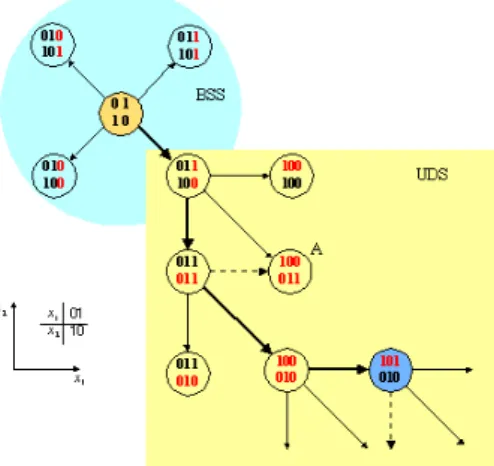
In this paper DEAS is applied to find optimal SVM param-eters which affect the performance of SVM, gradient descent method is used to find more exact values of parameters. Dynamic encoding algorithm for search (DEAS) proposed in [2] is based on dynamic binary string encoding for parame-ters. It is basically consists of Bi-sectional search (BSS) step and Unidirectional search (UDS) step. BSS step is a step for finding better parameter values and directions of UDS using bisectional search increasing coding length that increases the resolution of parameters. UDS is a searching step which fol-lows the directions decided in BSS step with out increasing code length.
Brief introductions of SVM and radius margin bound and it´s derivatives are given in Section 2, and the basic concepts of DEAS are explained in Section 3. In Section 4, proposed method is explained. The experimental result and discus-sion are described in the Section 5, In section 6, this paper summarize the conclusions.
2. Support Vector Machine
SVM is a binary classification algorithm based on statistical learning theory. The purpose of this algorithm is to make classifiers that produces desired output for given training data set LN = {(xi, yi)}i=0,...,N, where N is the number of
training set , xiis ith input vector and yi∈ {−1, +1} is ith
output that denotes the desired output class. The output value is based on the following decision function [6]:
f (x) = N X i=1 (yiα0iK(xi, x)) + b, (1) where α0
i ≥ 0 is the Lagrangian multiplier, b is bias term
and K(xi, xj) is kernel function that maps the input vectors
to the feature space. For given training data set L, finding the α0
i, i = 0..N which satisfy the output yiwith respect to
x is SVM training problem. α0 can be obtained by solving
the following quadratic optimization problem [8]: min α W (α) = minα { N X i=1 αi− N X i,j=1 αiαjyiyjK(xi, xj)} (2)
with constraints subject to 0 ≤ αi and
N
X
i=1
αiyi= 0, i = 1, ...., N (3)
and for every input xi, f (xi) satisfies yif (xi) ≥ 1 this
for-mulation is hard margin SVM optimization problem formu-lation. In hard margin formulation, no training errors are allowed.
2.1. Soft margin form
However, if there exist non-separable inputs what is called slack vector, it is needed to allowed training error which results soft margin algorithm. However, it can be considered as a special case of a hard margin form with the modified kernel [5][4]:
˜
K(xi, xj) = K(xi, xj) + 1
Cδij, (4)
where δij= 1 when i = j and δij= 0 when otherwise. Then
that controls the tradeoff between complexity of the decision function and the number of the training inputs that miss classified [7].
There are many different types of kernel functions. However the Popular choices of kernel functions are
Gaussian kernel : K(x, y) = exp
µ −kx − yk 2 2 2σ2 ¶ (5) P olynomial kernel : K(x, y) = ³ 1 +x · y σ2 ´d . (6)
In this paper, the Gaussian kernel is used for calculation and experiment.
2.2. Radius/margin bound
The performance of the SVM classifiers are described as the generalization error rate that is the error rate of input data set which is not included in training set. There are mainly two types of performance estimate are exist, single validation estimate leave-one-out and bounds.
If there exist enough data available, which called validation set, it is possible to estimate the true error rate. the sin-gle validation error T [5], for the given validation data set
{(xj, yj)}, i = 1, ..., p, T =1 p p X i=1 Ψ(−yif (xi)), (7)
where Ψ is a step function and p is the number of valida-tion set. While the Leave-one-out procedure, for the data set removing one element and training the SVM with the re-mained data and test the removed input data element. but it required large computation time if the number of a training data are large. These two estimations of the generalization performance are not easy to analysis and hard to find the gra-dient with respect to the SVM parameters. However it was shown by Vapnik and Chapelle [5] that following inequality holds,
Leave−One−Out error rate ≤ T = 1
N R2 γ2 = 1 NR 2 k w k22 (8) where R is the radius of smallest sphere enclosing the train-ing points mapped into a high dimensional feature space , w is a weight vector and γ is the margin. Thus, to minimize the T , one have to maximize the γ2 and minimize the R2.
To maximize the margin γ2, minimize the 2-norm of weight
vector k w k2
2, the norm of w∗, which is the optimal w, [6]
1 γ2 =k w k 2 2= N X i,j=0 yiyjα0iα0jK(xe i, xj) = N X i=0 α0 i−1 C < α 0•α0> . (9) The radius R can be obtained by solving following equation [8][4]: R2= N X i=1 βi0K(xe i, xj) − N X i,j=0 βi0β0jK(xe i, xj) (10) where the β0
i is the solution of following quadratic
optimiza-tion problem, min β Ã N X i=1 βiK(xe i, xj) − N X i,j=0 βiβjK(xe i, xj) ! , (11)
with constraints subject to
N
X
i=1
βi= 1, βi≥ 0. (12)
If there exist slack vectors, the radius/margin bound of the generalization error can be rewritten as in terms of 2-norm of a slack variables [6]. R2+ kξk22 kwk2 2 γ2 = k w k 2 2 µ R2+ k ξ k22 k w k2 2 ¶ (13) = k w k2 2R2+ k ξ k22, (14)
where ξ is a vector of the slack variables that satisfies Karush-Kuhn-Tucker complementary condition:
αi[yi(< w • xi> +b) − 1 + ξi] = 0, i = 1, ..., N. (15)
The properties of the bound given in equation (14), will be discussed in the experiment and discussion section, section 5.. 2.3. Derivative of radius margin bound
In most case, finding the gradient with respect to the SVM parameters (C, σ2) of radius/margin bound requirers
expen-sive matrix operations involving the kernel matrix. Thus, this paper consider only the Gaussian kernel function given by (5), because it is relatively easy to find the gradient of T , the radius/margin bound. The gradients of the ra-dius/margin bound are calculated in [5] as following equa-tions: ∂T ∂C = 1 N · ∂ k w k2 2 ∂C R 2 + k w k22 ∂R2 ∂C ¸ (16) ∂T ∂σ2 = 1 N · ∂ k w k2 2 ∂σ2 R 2 + k w k22 ∂R2 ∂σ2 ¸ . (17) The derivatives of k w k2 2 are as follows [1]: ∂ k w k2 2 ∂C = N X i=1 α2 i C2 (18) ∂ k w k2 2 ∂σ2 = − N X i,j=1 αiαjyiyj∂ e K(xi, xj) ∂σ2 (19)
and the derivatives of R2 are as follows:
∂R2 ∂C = − N X i=1 βi(1 − βi) C2 (20) ∂R2 ∂σ2 = − N X i,j=1 βiβj∂ e K(xi, xj) ∂σ2 . (21)
The derivative of the kernel with respect to σ2is
∂K(xe i, xj)
∂σ2 =K(xe i, xj)
k xi− xjk22
2σ4 . (22)
Thus, the gradient of the radius/margin bound is easily com-puted(because k w k2
3. DEAS
DEAS basically consists of two procedures: bisectional search(BSS) and unidirectional search(UDS). In the BSS step, the length of binary code is extended by 1 and the resolution of parameters is increased. The behavior of the BSS is explained about 1 and 2 dimensional case in Figure 1. By using the BSS, the minimum value of the a function for the parameterized code is found and also determined the direction of the UDS [2]. Figure 2. shows the UDS step after
Fig. 1. Bisectional search(BSS).
a BSS step in a 2-dimensional parameter space. The direc-tion found by the BSS step reflects descending tendency of the cost function. Thus, in a UDS steps, the evaluation of the cost function continues, until there are no smaller costs than the current minimum cost value, along the given di-rection. In the UDS steps, the length of the binary code is preserved while the binary code values increase or decrease [3]. The binary codes correspond to the values in a
normal-Fig. 2. Unidirectional search(UDS).
ized parameter space. The encoding of the binary code is given in Figure 3. Other encodings are also possible. For more detailed information refer [2][3].
4. SVM parameter optimization using DEAS and gradient descent method
The proposed method is a SVM parameter tuning frame-work based on DEAS and gradient descent method as an option. This method uses DEAS to find optimal values for the given resolution (length of binary string). For the candi-dates of optimal found by DEAS, gradient descent method
Fig. 3. Binary value encoding.
is applied to get more optimal solution. This framework for SVM parameter tuning is written in simple pseudo code:
1. Select the ranges of SVM parameters.
2. Select starting and terminating resolution of DEAS as the binary coding length (s,m) and determine the parameter resolution tolerance e.
3. Using DEAS, find the local optimal values for the given target resolution of DEAS.
4. For the candidate of optimal values found by DEAS If: 1
2m+1−1 ≤ e then, stop.
Else: start gradient descent method. 5. Save the optimal value and exit the algorithm. There were some earlier works on the SVM parameter op-timization. They used generally gradient descent method [5][1] or GA with gradient descent method [4]. In compar-ison with other method, the proposed method has several advantages.
First, it has less probability to fail in finding optimal pa-rameters or to get stuck in local minimum in comparison with gradient descent based method [1]. Since proposed method starts in many starting points, it has less probabil-ity to fail in finding optimal parameters. One can say that if the gradient descent method also can have multi starting points. However, if that strategy is applied to the gradient descent method, there will be many unnecessary gradient calculations around the minimum. In contrast with gradient descent method, DEAS has revisit check procedure for the calculated point and terminate that iteration to avoid over-lapping of searching area. Second, if the target resolution is sufficiently fine, there is no need to calculate the gradient of the radius/margin bound with respect to the SVM param-eters. Thus it is useful when tuning the SVM parameters which is applied other kernels and other bounds. In many cases, the calculation of the gradient of radius/margin bound requires expensive matrix calculations involving kernel ma-trix KN ×N.
GA based gradient descent algorithm was proposed in [4]. However, GA based on randomness of mutation, therefor, large computation time is required for little enhancement of performance. Thus, the computational requirement of DEAS is much less than the GA based algorithm. More over, DEAS has a strategy for the faster convergence to the minimum that makes DEAS more efficient searching algorithm.
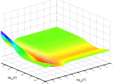
−1 −0.5 0 0.5 1 1.5 2 −4 −3 −2 −1 0 1 2 3 4 5 6 log10(σ 2 ) log10(C)
Fig. 4. The radius/margin bounds with the equation (14) for separating ’1’ form ’2’.
5. Experimental Result and discussion In this experiment, MNI steel hand-written character data are used. Table 1 shows the data which used in the SVM parameter tuning experiment. The error rate and the radius margin bounds with respect to the parameters are plotted on Figure 4., Figure 5. and Figure 6. Figure 4.,5. and 6. shows the error rate and bound for the first case in Table 1. The Figure 4. is a graph of the modified radius/margin bound which is related with equation (14) in [6]. Figure 5. is a graph of the radius/margin bound in the equation (8), and the Figure 6. is a graph of the error rate for the training data. −1 0 1 2 3 −4 −2 0 2 4 6 −6 −4 −2 0 2 log10(σ2)
radius margin boud for seperating ’1’ and ’2’
log10(C)
log10(R
2||w|| 2)
Fig. 5. The radius/margin bounds with the equation (8) for separating ’1’ form ’2’.
In these figures, one can see that the radius/magin bound based on the equation (14) shows better estimation for the error rate on this SVM parameter tuning problem than based on the equation (8) Thus, this paper use the modified radius margin form which makes slightly different the gradient form. However, it is easy to obtain the gradient when using 2-norm
Training and test data
training data number of number of test training data vectors class-1 class+1 class-1 class+1 class-1 class+1
’1’ ’2’ 20 20 100 100
’4’ ’9’ 20 20 100 100
’7’ ’9’ 20 20 100 100
’7’ ’8’ and ’0’ 40 20+20 100 200 Table 1. The size of the training and test data.
−1 0 1 2 3 −4 −2 0 2 4 6 −2 −1 0 1 log10(σ2)
error rate for seperating ’1’ and ’2’
log10(C)
log10(error rate)
Fig. 6. The error rate for training set for separating ’1’ form ’2’. −1 −0.5 0 0.5 1 1.5 2 −4 −3 −2 −1 0 1 2 3 4 5 6 log 10(σ 2) log 10(C)
Fig. 7. The radius/magin bound for separating ’7’ from ’8’ and ’0’.
soft margin form of the SVM with the condition αi = Cξi
[6]. Then, the gradient of the radius/margin bound changes as follows: ∂T ∂C = 1 N · ∂ k w k2 2 ∂C R 2+ k w k2 2 ∂R2 ∂C + ∂ k ξ k2 2 ∂C ¸ (23) = 1 N " ∂ k w k2 2 ∂C R 2 + k w k22 ∂R2 ∂C + −2 C3 N X i=1 αi # (24) ∂T ∂σ2 = 1 N · ∂ k w k2 2 ∂σ2 R 2 + k w k22 ∂R2 ∂σ2 ¸ . (25)
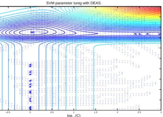
For given data sets in Table 1, DEAS is applied for parameter optimization. The result of of DEAS is shown in Table 2. The staring length of binary code of DEAS is 5 and the target length is 10. For efficiency, 100 starting points are selected randomly. Figure 9. shows the results and the characteristics
−1 0 1 2 3 −4 −2 0 2 4 6 −2 −1.5 −1 −0.5 0 0.5 1 log10(σ2 ) error rate for separating ’7’ and ’0’,’8’
log10(C)
log10(error rate)
Fig. 8. The test error rate for separating ’7’ from ’8’ and ’0’.
SVM parameter tunig with DEAS.
log10(C)
−0.5 0 0.5 1 1.5 2 2.5 3
Fig. 9. Applying DEAS on SVM parameter optimization that separate ’7’ from ’8’ and ’0’.
Fig. 10. Applying DEAS with starting resoution 4 and target resolution 6 and gradient descent method on a SVM parameter optimization that separate ’4’ from ’9’ . 0.02 0.025 0.03 0.035 0.04 0.045 0.05 3.3 3.305 3.31 3.315 3.32 3.325 3.33 −0.4377 −0.4376 −0.4375 −0.4374 −0.4373 −0.4372 log 10(C)
gradient decent method after DEAS with 10e−15 tolerance in variable
log 10(σ 2) log 10 (1/N(R ||w|| +|| ξ || ))
Fig. 11. Applying gradient descent method after DEAS on a SVM parameter optimization that separate ’4’ from ’9’.
separating data sets ’1’-’2’ ’4’-’9’ ’7’-’9’ ’7’-’0’&’8’ σ2 2.050350 e+003 2.144758 e+003 1.530209 e+003 3.421737 e+003 C 1.077105 e+000 1.106594 e+000 1.077105 e+000 1.181427 e+000 rasius mar-gin bound 2.503370 e-001 3.649682 e-001 3.860656 e-001 1.991583 e-001 errorate 5.500000 e-002 2.300000 e-001 1.500000 e-001 4.333333 e-002 evaluation count 2595 2622 2500 2741 Table 2. Optimal values found by DEAS only with starting resolution 5 and target resolution 10.
of DEAS for given data set(’7’-’0’,’8’). The dots denote the parameter point that the values of radius/margin bound is evaluated.
Figure 10. and 11. show the example of hybrid method, DEAS and gradient descent method. The start length of binary code of DEAS is 4 and the target length is 6. After DEAS, gradient descent method is applied to the result fount by DEAS. The result is shown in Table 3. The radius/margin is improved than the radius margin bound in Table 1 with less evaluation of the radius/margin bound. If the resolutions of the parameters are sufficiently fine, the iteration step of DEAS is completed. If the resolution of the parameters is not sufficiently fine, additional gradient descent step is executed. Since the bound is rough, the SVM parameter found by the radius/margin bound is close to optimal , but not optimal in practice.
However, it is possible to find the optimal parameters using the training error with DEAS, for reasonable size of subset of a test data with respect to the SVM parameters. Proposed method can be used in parameter tuning with test errors that are generally discrete with respect to the parameters. More over, it requires much less computation time than the GA or other searching methods based on randomness.
’4’-’9’ with DEAS ’4’-’9’ with gradient descent method after DEAS
sigma2 2.002568e+003 2.132606e+003
C 1.037225e+000 1.105078e+000 radius margin
bound
3.654323e-001 3.649664e-001 error rate 2.250000e-001 2.300000e-001 Table 3. Parameter optimizing using both DEAS and the gradient descent method
6. conclusion
This paper shows that the radius/margin bound is gener-ally rough. Moreover, the optimal parameter value which is found by using the radius/margin bound can converge or di-verge into unreasonable value. To overcome the drawback of using radius/margin bound, the radius margin bound equa-tion changed (8) to (14) . This paper also propose an efficient method for the SVM parameter tuning method using DEAS, even if gradient information is not available. If it is avail-able, using a hybrid strategy which controls the resolution of DEAS and uses the gradient decent method, one can find the optimal value more efficiently.
References
[1] S.S. Keerthi. Efficient tuning of svm hyperparameters using radius/margin. IEEE Transactions on Neural
Net-works, 13:1225–1229, 2002.
[2] Jong-Wook Kim & Sang Woo Kim. Numerical method for global optimization: Dynamic encoding algorithm for searches. IEE proc.- Control Theory & Appl., 151(5):661– 668, Sept. 2004.
[3] Nam Gun Kim & Jong-Wook Kim & Sang Woo Kim. A study for global optimization using dynamic encoding algoritm for searches. ICCAS, pages 857–862, 2004. [4] Abhijit Kulkarni & V. K. Jayaraman & B. D. Kulkarni.
Support vector classification with parameter tuning as-sisted by agent-based technique. Computers & Chemical
Engineering, pages 311–318, 2004.
[5] Olivier Chapelle & Vladimir Vapnik & Olivier Bousquet & Sayan Mukherjee. Choosing multiple parameters for support vector machines. Mach. Learn., 46(1-3):131–159, 2002.
[6] N. Cristianini & J. Shawe-Taylor. An introduction to
Support Vector Machies. Cambridge University Press,
2000.
[7] O. Chapelle & V. Vapnik. Model selection for support vector machies. Advances in Neural Information
Process-ing systems, pages 230–236, 1999.
[8] V. Vapnik. Statiscal Learning Theory. Weily, 1998. [9] V. Vapnik and O. chapelle. Bounds on error expectation