A Generalized Finite Difference Method for Solving Fokker-Planck-Kolmogorov Equations

(1)

816 http://ijass.org pISSN: 2093-274x eISSN: 2093-2480

Paper

Int’l J. of Aeronautical & Space Sci. 18(4), 816–826 (2017) DOI: http://dx.doi.org/10.5139/IJASS.2017.18.4.816

A Generalized Finite Difference Method for Solving

Fokker-Planck-Kol-mogorov Equations

Li Zhao*

Department of Civil Engineering, The University of Akron, 44325, OH, USA

Gun Jin Yun**

Department of Mechanical and Aerospace Engineering, Seoul National University, Seoul 08826, Republic of Korea

Abstract

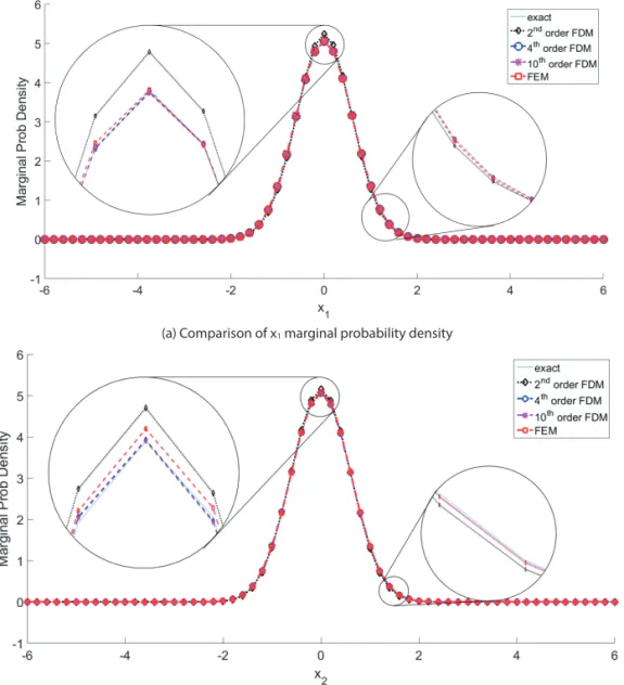
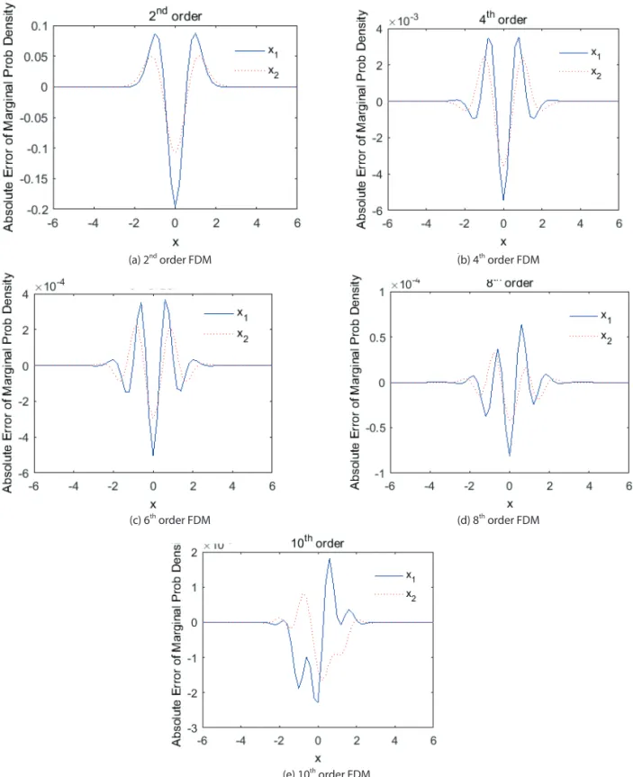
In this paper, a generalized discretization scheme is proposed that can derive general-order finite difference equations representing the joint probability density function of dynamic response of stochastic systems. The various order of finite difference equations are applied to solutions of the Fokker-Planck-Kolmogorov (FPK) equation. The finite difference equations derived by the proposed method can greatly increase accuracy even at the tail parts of the probability density function, giving accurate reliability estimations. Compared with exact solutions and finite element solutions, the generalized finite difference method showed increasing accuracy as the order increases. With the proposed method, it is allowed to use different orders and types (i.e. forward, central or backward) of discretization in the finite difference method to solve FPK and other partial differential equations in various engineering fields having requirements of accuracy or specific boundary conditions.

Key words: Fokker-Planck-Kolmogorov equation, Finite difference method, Stochastic differential equation, Random vibration

1. Introduction

The response and reliability of engineering structures subjected to random excitations has long been interests to researchers and studied through stochastic approaches for many years. For example, pressure fields generated inside of jet and rocket propulsion is a complicated random process that creates vibration to aircraft and missile structures. Random response of multi-dimensional linear dynamic systems can be found in Nigam [1]. Caughey reported that random response of memoryless dynamic systems can be obtained as a solution of the forward Fokker-Planck and backward Kolmogorov equations [2]. A linear system subjected to additive Gaussian random excitations shows Gaussian response. It is well known that the response of a random dynamic system is a Markov (Brownian motion) process (Xt), and can be governed by an

Ito stochastic differential equation (SDE) as below

1. Introduction

The response and reliability of engineering structures subjected to random excitations has long been interests to researchers and studied through stochastic approaches for many years. For example, pressure fields generated inside of jet and rocket propulsion is a complicated random process that creates vibration to aircraft and missile structures. Random response of multi-dimensional linear dynamic systems can be found in Nigam [1]. Caughey reported that random response of memoryless dynamic systems can be obtained as a solution of the forward Fokker-Planck and backward Kolmogorov equations [2]. A linear system subjected to additive Gaussian random excitations shows Gaussian response. It is well known that the response of a random dynamic system is a Markov (Brownian motion) process (𝑿𝑿𝑿𝑿𝑡𝑡𝑡𝑡), and can

be governed by an Ito stochastic differential equation (SDE) as below

𝑑𝑑𝑑𝑑𝑿𝑿𝑿𝑿𝑡𝑡𝑡𝑡= 𝑨𝑨𝑨𝑨(𝑿𝑿𝑿𝑿𝑡𝑡𝑡𝑡, 𝑡𝑡𝑡𝑡)𝑑𝑑𝑑𝑑𝑡𝑡𝑡𝑡 + 𝑩𝑩𝑩𝑩(𝑿𝑿𝑿𝑿𝑡𝑡𝑡𝑡, 𝑡𝑡𝑡𝑡)𝑑𝑑𝑑𝑑𝑾𝑾𝑾𝑾(𝑡𝑡𝑡𝑡) , (1)

where 𝑨𝑨𝑨𝑨(𝑿𝑿𝑿𝑿𝑡𝑡𝑡𝑡, 𝑡𝑡𝑡𝑡) and 𝑩𝑩𝑩𝑩(𝑿𝑿𝑿𝑿𝑡𝑡𝑡𝑡, 𝑡𝑡𝑡𝑡) are the drift vector and diffusion matrix, respectively; 𝑾𝑾𝑾𝑾(𝑡𝑡𝑡𝑡)

is the Gaussian white noise vector (represented by Wiener process) having properties of < 𝑊𝑊𝑊𝑊𝑖𝑖𝑖𝑖(𝑡𝑡𝑡𝑡) >= 0, < 𝑊𝑊𝑊𝑊𝑖𝑖𝑖𝑖(𝑡𝑡𝑡𝑡1)𝑊𝑊𝑊𝑊𝑗𝑗𝑗𝑗(𝑡𝑡𝑡𝑡1+ 𝜏𝜏𝜏𝜏) >= 2𝐷𝐷𝐷𝐷𝑖𝑖𝑖𝑖𝑗𝑗𝑗𝑗𝛿𝛿𝛿𝛿(𝜏𝜏𝜏𝜏) , (2)

< 𝑑𝑑𝑑𝑑𝑾𝑾𝑾𝑾(𝑡𝑡𝑡𝑡)𝑑𝑑𝑑𝑑𝑾𝑾𝑾𝑾(𝑡𝑡𝑡𝑡)𝑇𝑇𝑇𝑇_{>= 𝑰𝑰𝑰𝑰𝑑𝑑𝑑𝑑𝑡𝑡𝑡𝑡 ,} ₍₃₎

where <∙> is the expectation operator; 𝛿𝛿𝛿𝛿(∙) is the Dirac delta function; and 𝐷𝐷𝐷𝐷𝑖𝑖𝑖𝑖𝑗𝑗𝑗𝑗/𝜋𝜋𝜋𝜋 is the

amplitude of the constant two-sided power spectral density of the random input; and 𝑰𝑰𝑰𝑰 is the identity matrix. This process can be determined by the transitional probability density function (PDF) which satisfies both forward Kolmogorov equation, also called Fokker-Planck-Kolmogorov (FPK) equation and backward Kolmogorov equation. Equivalency of Ito SDE to FPK equation is explained in appendix of this paper. The transitional PDF of the response can be obtained by solving the corresponding FPK equation.

The earliest numerical method used to solve FPK equations was finite difference

, (1)

where A(Xt , t) and B(Xt , t) are the drift vector and diffusion

matrix, respectively; W(t) is the Gaussian white noise vector (represented by Wiener process) having properties of

1. Introduction

𝑑𝑑𝑑𝑑𝑿𝑿𝑿𝑿𝑡𝑡𝑡𝑡= 𝑨𝑨𝑨𝑨(𝑿𝑿𝑿𝑿𝑡𝑡𝑡𝑡, 𝑡𝑡𝑡𝑡)𝑑𝑑𝑑𝑑𝑡𝑡𝑡𝑡 + 𝑩𝑩𝑩𝑩(𝑿𝑿𝑿𝑿𝑡𝑡𝑡𝑡, 𝑡𝑡𝑡𝑡)𝑑𝑑𝑑𝑑𝑾𝑾𝑾𝑾(𝑡𝑡𝑡𝑡) , (1)

< 𝑑𝑑𝑑𝑑𝑾𝑾𝑾𝑾(𝑡𝑡𝑡𝑡)𝑑𝑑𝑑𝑑𝑾𝑾𝑾𝑾(𝑡𝑡𝑡𝑡)𝑇𝑇𝑇𝑇_{>= 𝑰𝑰𝑰𝑰𝑑𝑑𝑑𝑑𝑡𝑡𝑡𝑡 ,} ₍₃₎

2

, (2)

1. Introduction

𝑑𝑑𝑑𝑑𝑿𝑿𝑿𝑿𝑡𝑡𝑡𝑡 = 𝑨𝑨𝑨𝑨(𝑿𝑿𝑿𝑿𝑡𝑡𝑡𝑡, 𝑡𝑡𝑡𝑡)𝑑𝑑𝑑𝑑𝑡𝑡𝑡𝑡 + 𝑩𝑩𝑩𝑩(𝑿𝑿𝑿𝑿𝑡𝑡𝑡𝑡, 𝑡𝑡𝑡𝑡)𝑑𝑑𝑑𝑑𝑾𝑾𝑾𝑾(𝑡𝑡𝑡𝑡) , (1)

< 𝑑𝑑𝑑𝑑𝑾𝑾𝑾𝑾(𝑡𝑡𝑡𝑡)𝑑𝑑𝑑𝑑𝑾𝑾𝑾𝑾(𝑡𝑡𝑡𝑡)𝑇𝑇𝑇𝑇 _{>= 𝑰𝑰𝑰𝑰𝑑𝑑𝑑𝑑𝑡𝑡𝑡𝑡 ,} ₍₃₎

2

, (3)

where <∙> is the expectation operator; δ(∙) is the Dirac delta function; and Dij/π is the amplitude of the constant

two-sided power spectral density of the random input; and I is the identity matrix. This process can be determined by the transitional probability density function (PDF) which satisfies both forward Kolmogorov equation, also called Fokker-Planck-Kolmogorov (FPK) equation and backward Fokker-Planck-Kolmogorov equation. Equivalency of Ito SDE to FPK equation is explained in appendix of this paper. The transitional PDF of the response can be obtained by solving the corresponding FPK equation.

The earliest numerical method used to solve FPK equations was finite difference method (FDM). In 1969, Chang and Cooper

This is an Open Access article distributed under the terms of the Creative Com-mons Attribution Non-Commercial License (http://creativecomCom-mons.org/licenses/by- (http://creativecommons.org/licenses/by-nc/3.0/) which permits unrestricted non-commercial use, distribution, and reproduc-tion in any medium, provided the original work is properly cited.

* Ph. D Student

** Professor, Corresponding author: [email protected]

(2)

817

Li Zhao A Generalized Finite Difference Method for Solving Fokker-Planck-Kolmogorov Equations

http://ijass.org [3] firstly developed a finite difference scheme to solve

one-dimensional FPK equations. This scheme not only satisfies both convergence and unconditional stability conditions, but also preserve properties of the original partial differential equation especially non-negativity. Later, Roberts [4] applied an implicit finite difference approximation to predict two-dimensional first-passage failure probability for oscillators under stationary wide-band random excitation. Zorzano et al. [5] also used the FDM to solve transient FPK problems and compared the results with exact solutions, showing good accuracy. With the inherent advantage of stability, finite element method (FEM) was also applied to approximate the solution of FPK equations. Langley [6] derived a weak form of the stationary FPK equation by integration-by-part and then successfully used FEM to compute numerical solutions of the stationary PDF of the random response. Langtangen [7] extended Langley’s work of FEM in more details and contributed a stronger mathematical foundation to this method. Later in 1993, Bergman and Spencer [8] applied FEM to solve two-dimensional transient FPK equation for stochastic dynamic systems for the first time and gave the joint probability density function (JPDF) of responses under a given initial condition. Results were also compared with those from backward equations showing high accuracy. Path integral solution method was also applied to solve FPK equations [9-11]. The path integral solution approaches based on a discretized version of the Chapman-Kolmogorov equation proved to be very accurate for linear SDOF systems [12]. Importance of accurate approximations of tail parts of transitional PDF in reliability analysis was addressed when the path integral solution method was used [13; 14].

The first-order FDM and FEM aforementioned are able to give solutions of the FPK equation with good accuracy (i.e. O(10-4_{)), which is, however, sometimes not acceptable in the}

tail parts of the computed probability distribution. To improve the accuracy, Wojtkiewicz et al. [15] proposed use of a high-order FDM that can give higher accuracy even at the tail of the probability distribution for the second-order FPK system response. Although the authors later pointed out that this scheme carried inherent stability issue and required refinement of mesh, which impeded the progress of extending this scheme for solving three or higher dimensional FPK problems, the substantial enhancement of accuracy still made the high-order FDM an important numerical method to solve FPK equations. Kumar and Narayanan [16] applied both the FEM and high-order FDM to solve a stochastic system and confirmed the advantage of the high-order FDM in achieving higher accuracy. A generalized difference scheme was applied to direct time integration method for structural dynamics problems [17].

In this paper, a generalization of the high-order difference

scheme in the response domain of FPK problems is proposed for the first time. In previous applications of the high-order FDM for solving FPK, only equations for second, fourth, sixth, and eighth-order central discretization approximation for derivatives (e.g. ∂P/∂x, (∂2_P)/(∂x2_{)) were given [15]. There}

has been no generalized method that allows for generating discretization of different orders and types (i.e. forward, central or backward) to approximate derivatives (e.g.

∂P/∂x, (∂2_P)/(∂x2_{)) according to the specific requirements}

of accuracy or different boundary conditions, which will undoubtedly limit the application and extension of the high-order method to solve various FPK problems depending on users’ needs. It will be illustrated that the high-order central discretization used by Wojtkiewicz et al. [15] is a special case of the proposed generalized difference method. Then, the generalized high-order FDM will be applied to solve a two-dimensional linear random dynamic system. The results are compared not only with those from FEM but also the exact solution, showing significant promise in improving the accuracy. This generalization of the high-order FDM provides a strong theoretical basis for further study of the FDM using different discretization scheme such as high-order forward, central or backward depending on users’ needs.

2. Generalization of Difference Discretization

of Probabilistic Density Function

In this section, a generalization theory was proposed to achieve a generalized discretization scheme to approximate transitional PDF and its derivatives with different orders and types of the approximation. The purpose of this generalization is to obtain a consistent method for deriving recurrence relations, which are not dependent on variations of the PDF and its derivatives within the response domain. In the end, the first and second order derivatives of the PDF in FPK equations were replaced with discrete values of PDF at n response points.

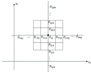
The response domain in x is discretized into n nodes resulting in n discrete approximations of p(x1), p(x2), p(x3),

…, p(xn-1), and p(xn) to the PDF P. The normalized location X

can be defined by

2. Generalization of Difference Discretization of Probabilistic Density Function

In this section, a generalization theory was proposed to achieve a generalized discretization scheme to approximate transitional PDF and its derivatives with different orders and types of the approximation. The purpose of this generalization is to obtain a consistent method for deriving recurrence relations, which are not dependent on variations of the PDF and its derivatives within the response domain. In the end, the first and second order derivatives of the PDF in FPK equations were replaced with discrete values of PDF at n response points. The response domain in x is discretized into n nodes resulting in n discrete approximations of p(x1), p(x2), p(x3), …, p(xn−1), and p(xn) to the PDF P. The normalized location X

can be defined by

X = (x − x0)/dx , (4)

where x0is the origin of the x response domain. x0 can be any node in the response domain.

Then, a basic generalized difference equation for derivatives of the PDF P at X = 0 (i.e. the origin where x = x0) is defined as

Pj_(0)dxj_{= ∑} _a

ji p(xk+1−i) n−1

i=0 for j = 0, … , n − 1 , (5)

where Pj_{(0) is the j}th_{derivative of the probability density at the origin x = x}

0 (i.e. X = 0)

and p(xk+1−i) is the approximation of P at xk+1−i. We let [18; 19]

p(xk+1−i) = fm(Xi) , i = 0,1, … . , n − 1 , (6)

fm(Xi) = ∑mj=0_j!1bj(x − x0)j, m = 0,1, … . , n − 1 . (7)

The assumed p(xk+1−i) in Eq. (5) should be able to ensure that the jthorder derivative of the

probability density Pj _{at all nodes can be a constant value, which is called the consistency}

condition. In order to force p(xk+1−i) to satisfy the consistency condition, the following

equation can be formed [18; 19]:

, (4)

where x0 is the origin of the x response domain. x0 can be

any node in the response domain. Then, a basic generalized difference equation for derivatives of the PDF P at X=0 (i.e. the origin where x= x0) is defined as

can be defined by

X = (x − x0)/dx , (4)

Pj_(0)dxj_{= ∑} _a

i=0 for j = 0, … , n − 1 , (5)

0 (i.e. X = 0)

p(xk+1−i) = fm(Xi) , i = 0,1, … . , n − 1 , (6)

fm(Xi) = ∑mj=0_j!1bj(x − x0)j, m = 0,1, … . , n − 1 . (7)

5

can be defined by

X = (x − x0)/dx , (4)

where x0 is the origin of the x response domain. x0 can be any node in the response domain.

Pj_(0)dxj_{= ∑} _a

i=0 for j = 0, … , n − 1 , (5)

0 (i.e. X = 0)

p(xk+1−i) = fm(Xi) , i = 0,1, … . , n − 1 , (6)

fm(Xi) = ∑mj=0_j!1bj(x − x0)j, m = 0,1, … . , n − 1 . (7)

,

(5)

(3)

DOI: http://dx.doi.org/10.5139/IJASS.2017.18.4.816 ₈₁₈

Int’l J. of Aeronautical & Space Sci. 18(4), 816–826 (2017)

where Pj_{(0) is the j}th_{derivative of the probability density at}

the origin x=x0 (i.e. X=0) and p(xk+1-i) is the approximation of

P at xk+1-i. We let [18; 19]

can be defined by

X = (x − x0)/dx , (4)

Pj_(0)dxj_{= ∑} _a

i=0 for j = 0, … , n − 1 , (5)

0 (i.e. X = 0)

p(xk+1−i) = fm(Xi) , i = 0,1, … . , n − 1 , (6)

fm(Xi) = ∑mj=0_j!1bj(x − x0)j, m = 0,1, … . , n − 1 . (7)

5

, (6)

can be defined by

X = (x − x0)/dx , (4)

Pj_(0)dxj_{= ∑} _a

i=0 for j = 0, … , n − 1 , (5)

0 (i.e. X = 0)

p(xk+1−i) = fm(Xi) , i = 0,1, … . , n − 1 , (6)

fm(Xi) = ∑mj=0_j!1bj(x − x0)j, m = 0,1, … . , n − 1 . (7)

5

. (7)

The assumed p(xk+1-i) in Eq. (5) should be able to ensure

that the jth_{order derivative of the probability density P}j_{at all}

nodes can be a constant value, which is called the consistency condition. In order to force p(xk+1-i) to satisfy the consistency

condition, the following equation can be formed [18; 19]:

6 [ 1 … 1 X0 … Xn−1 ⋮ ⋮ ⋮ ⋮ ⋮ ⋮ X0n−1 … Xn−1n−1][ 𝑎𝑎00 … 𝑎𝑎𝑛𝑛−1,0 𝑎𝑎01 … 𝑎𝑎𝑛𝑛−1,1 ⋮ ⋮ ⋮ ⋮ ⋮ ⋮ 𝑎𝑎0,𝑛𝑛−1 … 𝑎𝑎𝑛𝑛−1,𝑛𝑛−1] = [ 1 ₁ 2! ⋱ ⋱ (𝑛𝑛 − 1)! ] or [𝑉𝑉𝑛𝑛][𝐴𝐴𝑛𝑛] = [𝐸𝐸𝑛𝑛] (8)

where [𝐴𝐴𝑛𝑛] is the coefficient matrix and [𝑉𝑉𝑛𝑛] is known as Vandermonde matrix, which

depends on the choice of x0. By taking the inverse of [𝑉𝑉𝑛𝑛], [𝐴𝐴𝑛𝑛] can be calculated as follows

[𝐴𝐴𝑛𝑛] = [𝑉𝑉𝑛𝑛]−1[𝐸𝐸𝑛𝑛]. (9)

Then, according to Eq. (5), the jth_{derivative of P(0) can be obtained as an expression including}

coefficients [𝐴𝐴𝑛𝑛]. {Pj_{(0)} = [T][A} n]T{p} (10) Eq. (10) is expanded as { 𝑃𝑃_𝑃𝑃0₁(0)₍₀₎ . . . 𝑃𝑃𝑛𝑛−1_(0)} = [ 1 1 ∆𝑥𝑥 ⋱ ⋱ ⋱ _∆𝑥𝑥1_𝑛𝑛−1 _][ 𝑎𝑎00 … 𝑎𝑎0,𝑛𝑛−1 𝑎𝑎10 … 𝑎𝑎1,𝑛𝑛−1 ⋮ ⋮ ⋮ ⋮ ⋮ ⋮ 𝑎𝑎𝑛𝑛−1,0 … 𝑎𝑎𝑛𝑛−1,𝑛𝑛−1]{ 𝑝𝑝𝑘𝑘+1 𝑝𝑝𝑘𝑘 . . . 𝑝𝑝𝑘𝑘−𝑛𝑛+2} (11)

where the notation 𝑝𝑝𝑘𝑘+1 is used instead of 𝑝𝑝(𝑥𝑥𝑘𝑘+1) . From Eq. (11), up to (𝑛𝑛 − 1)𝑡𝑡ℎ

(8)

where [An] is the coefficient matrix and [Vn] is known as

Vandermonde matrix, which depends on the choice of x0. By

taking the inverse of [Vn], [An] can be calculated as follows

⎣ ⎢ ⎢ ⎢ ⎢ ⎡_X1 … 1₀ _{… X}_n−1 ⋮ ⋮ ⋮ ⋮ ⋮ ⋮ X0n−1 … Xn−1n−1⎦ ⎥ ⎥ ⎥ ⎥ ⎤ ⎣ ⎢ ⎢ ⎢ ⎢ ⎡ 𝑎𝑎𝑎𝑎_{𝑎𝑎𝑎𝑎}00₀₁ … 𝑎𝑎𝑎𝑎_{… 𝑎𝑎𝑎𝑎}𝑛𝑛𝑛𝑛−1,0_{𝑛𝑛𝑛𝑛−1,1} ⋮ ⋮ ⋮ ⋮ ⋮ ⋮ 𝑎𝑎𝑎𝑎0,𝑛𝑛𝑛𝑛−1 … 𝑎𝑎𝑎𝑎𝑛𝑛𝑛𝑛−1,𝑛𝑛𝑛𝑛−1⎦ ⎥ ⎥ ⎥ ⎥ ⎤ = ⎣ ⎢ ⎢ ⎢ ⎢ ⎡ 1 ₁ 2! ⋱ ⋱ (𝑛𝑛𝑛𝑛 − 1)!⎦⎥ ⎥ ⎥ ⎥ ⎤ or [𝑉𝑉𝑉𝑉𝑛𝑛𝑛𝑛][𝐴𝐴𝐴𝐴𝑛𝑛𝑛𝑛] = [𝐸𝐸𝐸𝐸𝑛𝑛𝑛𝑛] . (8)

where [𝐴𝐴𝐴𝐴𝑛𝑛𝑛𝑛] is the coefficient matrix and [𝑉𝑉𝑉𝑉𝑛𝑛𝑛𝑛] is known as Vandermonde matrix, which

depends on the choice of x0. By taking the inverse of [𝑉𝑉𝑉𝑉𝑛𝑛𝑛𝑛], [𝐴𝐴𝐴𝐴𝑛𝑛𝑛𝑛] can be calculated as

follows

[𝐴𝐴𝐴𝐴𝑛𝑛𝑛𝑛] = [𝑉𝑉𝑉𝑉𝑛𝑛𝑛𝑛]−1[𝐸𝐸𝐸𝐸𝑛𝑛𝑛𝑛]. (9)

Then, according to Eq. (5), the jth _{derivative of P(0) can be obtained as an expression}

including coefficients [𝐴𝐴𝐴𝐴𝑛𝑛𝑛𝑛]. �Pj_{(0)� = [T][A} n]T{p} . (10) Eq. (10) is expanded as ⎩ ⎪ ⎨ ⎪ ⎧ 𝜕𝜕𝜕𝜕_{𝜕𝜕𝜕𝜕}0₁(0)₍₀₎ . . . 𝜕𝜕𝜕𝜕𝑛𝑛𝑛𝑛−1_(0)⎭⎪ ⎬ ⎪ ⎫ = ⎣ ⎢ ⎢ ⎢ ⎢ ⎢ ⎡ 1 1 ∆𝑥𝑥𝑥𝑥 ⋱ ⋱ ⋱ _{∆𝑥𝑥𝑥𝑥}1𝑛𝑛𝑛𝑛−1 ⎦ ⎥ ⎥ ⎥ ⎥ ⎥ ⎤ ⎣ ⎢ ⎢ ⎢ ⎢ ⎡ 𝑎𝑎𝑎𝑎_{𝑎𝑎𝑎𝑎}00₁₀ … 𝑎𝑎𝑎𝑎_{… 𝑎𝑎𝑎𝑎}0,𝑛𝑛𝑛𝑛−1_{1,𝑛𝑛𝑛𝑛−1} ⋮ ⋮ ⋮ ⋮ ⋮ ⋮ 𝑎𝑎𝑎𝑎𝑛𝑛𝑛𝑛−1,0 … 𝑎𝑎𝑎𝑎𝑛𝑛𝑛𝑛−1,𝑛𝑛𝑛𝑛−1⎦ ⎥ ⎥ ⎥ ⎥ ⎤ ⎩ ⎪ ⎨ ⎪ ⎧ 𝑝𝑝𝑝𝑝_{𝑝𝑝𝑝𝑝}𝑘𝑘𝑘𝑘+1_{𝑘𝑘𝑘𝑘} . . . 𝑝𝑝𝑝𝑝𝑘𝑘𝑘𝑘−𝑛𝑛𝑛𝑛+2⎭ ⎪ ⎬ ⎪ ⎫ , (11) 6 . (9)

Then, according to Eq. (5), the jth derivative of P(0) can be obtained as an expression including coefficients [An].

⎣ ⎢ ⎢ ⎢ ⎢ ⎡_X1 … 1₀ _{… X}_n−1 ⋮ ⋮ ⋮ ⋮ ⋮ ⋮ X0n−1 … Xn−1n−1⎦ ⎥ ⎥ ⎥ ⎥ ⎤ ⎣ ⎢ ⎢ ⎢ ⎢ ⎡ 𝑎𝑎𝑎𝑎_{𝑎𝑎𝑎𝑎}00₀₁ … 𝑎𝑎𝑎𝑎_{… 𝑎𝑎𝑎𝑎}𝑛𝑛𝑛𝑛−1,0_{𝑛𝑛𝑛𝑛−1,1} ⋮ ⋮ ⋮ ⋮ ⋮ ⋮ 𝑎𝑎𝑎𝑎0,𝑛𝑛𝑛𝑛−1 … 𝑎𝑎𝑎𝑎𝑛𝑛𝑛𝑛−1,𝑛𝑛𝑛𝑛−1⎦ ⎥ ⎥ ⎥ ⎥ ⎤ = ⎣ ⎢ ⎢ ⎢ ⎢ ⎡ 1 ₁ 2! ⋱ ⋱ (𝑛𝑛𝑛𝑛 − 1)!⎦⎥ ⎥ ⎥ ⎥ ⎤ or [𝑉𝑉𝑉𝑉𝑛𝑛𝑛𝑛][𝐴𝐴𝐴𝐴𝑛𝑛𝑛𝑛] = [𝐸𝐸𝐸𝐸𝑛𝑛𝑛𝑛] . (8)

where [𝐴𝐴𝐴𝐴𝑛𝑛𝑛𝑛] is the coefficient matrix and [𝑉𝑉𝑉𝑉𝑛𝑛𝑛𝑛] is known as Vandermonde matrix, which

depends on the choice of x0. By taking the inverse of [𝑉𝑉𝑉𝑉𝑛𝑛𝑛𝑛], [𝐴𝐴𝐴𝐴𝑛𝑛𝑛𝑛] can be calculated as

follows

[𝐴𝐴𝐴𝐴𝑛𝑛𝑛𝑛] = [𝑉𝑉𝑉𝑉𝑛𝑛𝑛𝑛]−1[𝐸𝐸𝐸𝐸𝑛𝑛𝑛𝑛]. (9)

Then, according to Eq. (5), the jth _{derivative of P(0) can be obtained as an expression}

including coefficients [𝐴𝐴𝐴𝐴𝑛𝑛𝑛𝑛]. �Pj_{(0)� = [T][A} n]T{p} . (10) Eq. (10) is expanded as ⎩ ⎪ ⎨ ⎪ ⎧ 𝜕𝜕𝜕𝜕_{𝜕𝜕𝜕𝜕}0₁(0)₍₀₎ . . . 𝜕𝜕𝜕𝜕𝑛𝑛𝑛𝑛−1_(0)⎭⎪ ⎬ ⎪ ⎫ = ⎣ ⎢ ⎢ ⎢ ⎢ ⎢ ⎡ 1 1 ∆𝑥𝑥𝑥𝑥 ⋱ ⋱ ⋱ _{∆𝑥𝑥𝑥𝑥}1𝑛𝑛𝑛𝑛−1 ⎦ ⎥ ⎥ ⎥ ⎥ ⎥ ⎤ ⎣ ⎢ ⎢ ⎢ ⎢ ⎡ 𝑎𝑎𝑎𝑎_{𝑎𝑎𝑎𝑎}00₁₀ … 𝑎𝑎𝑎𝑎_{… 𝑎𝑎𝑎𝑎}0,𝑛𝑛𝑛𝑛−1_{1,𝑛𝑛𝑛𝑛−1} ⋮ ⋮ ⋮ ⋮ ⋮ ⋮ 𝑎𝑎𝑎𝑎𝑛𝑛𝑛𝑛−1,0 … 𝑎𝑎𝑎𝑎𝑛𝑛𝑛𝑛−1,𝑛𝑛𝑛𝑛−1⎦ ⎥ ⎥ ⎥ ⎥ ⎤ ⎩ ⎪ ⎨ ⎪ ⎧ 𝑝𝑝𝑝𝑝_{𝑝𝑝𝑝𝑝}𝑘𝑘𝑘𝑘+1_{𝑘𝑘𝑘𝑘} . . . 𝑝𝑝𝑝𝑝𝑘𝑘𝑘𝑘−𝑛𝑛𝑛𝑛+2⎭ ⎪ ⎬ ⎪ ⎫ , (11) 6 . (10) Eq. (10) is expanded as 6 [ 1 … 1 X0 … Xn−1 ⋮ ⋮ ⋮ ⋮ ⋮ ⋮ X0n−1 … Xn−1n−1][ 𝑎𝑎00 … 𝑎𝑎𝑛𝑛−1,0 𝑎𝑎01 … 𝑎𝑎𝑛𝑛−1,1 ⋮ ⋮ ⋮ ⋮ ⋮ ⋮ 𝑎𝑎0,𝑛𝑛−1 … 𝑎𝑎𝑛𝑛−1,𝑛𝑛−1] = [ 1 ₁ 2! ⋱ ⋱ (𝑛𝑛 − 1)! ] or [𝑉𝑉𝑛𝑛][𝐴𝐴𝑛𝑛] = [𝐸𝐸𝑛𝑛] (8)

where [𝐴𝐴𝑛𝑛] is the coefficient matrix and [𝑉𝑉𝑛𝑛] is known as Vandermonde matrix, which

depends on the choice of x0. By taking the inverse of [𝑉𝑉𝑛𝑛], [𝐴𝐴𝑛𝑛] can be calculated as follows

[𝐴𝐴𝑛𝑛] = [𝑉𝑉𝑛𝑛]−1[𝐸𝐸𝑛𝑛]. (9)

Then, according to Eq. (5), the jth_{derivative of P(0) can be obtained as an expression including}

coefficients [𝐴𝐴𝑛𝑛]. {Pj_{(0)} = [T][A}_n_]T_{p} ₍₁₀₎ Eq. (10) is expanded as { 𝑃𝑃_𝑃𝑃0₁(0)₍₀₎ . . . 𝑃𝑃𝑛𝑛−1_(0)} = [ 1 1 ∆𝑥𝑥 ⋱ ⋱ ⋱ _∆𝑥𝑥1𝑛𝑛−1 ][ 𝑎𝑎00 … 𝑎𝑎0,𝑛𝑛−1 𝑎𝑎10 … 𝑎𝑎1,𝑛𝑛−1 ⋮ ⋮ ⋮ ⋮ ⋮ ⋮ 𝑎𝑎𝑛𝑛−1,0 … 𝑎𝑎𝑛𝑛−1,𝑛𝑛−1]{ 𝑝𝑝𝑘𝑘+1 𝑝𝑝𝑘𝑘 . . . 𝑝𝑝𝑘𝑘−𝑛𝑛+2} (11)

where the notation 𝑝𝑝𝑘𝑘+1 is used instead of 𝑝𝑝(𝑥𝑥𝑘𝑘+1) . From Eq. (11), up to (𝑛𝑛 − 1)𝑡𝑡ℎ

(11)

where the notation pk+1 is used instead of p(xk+1). From Eq.

(11), up to (n-1)th_{derivatives of PDF can be written in}

terms of n discrete values of the PDF. Determination of the coefficients used in the generalized difference equation from consistency conditions is presented as an example for the case of n=3.

From Eq. (5),

where the notation 𝑝𝑝𝑝𝑝𝑘𝑘𝑘𝑘+1 is used instead of 𝑝𝑝𝑝𝑝(𝜕𝜕𝜕𝜕𝑘𝑘𝑘𝑘+1). From Eq. (11), up to (𝑛𝑛𝑛𝑛 − 1)𝑡𝑡𝑡𝑡ℎ

derivatives of PDF can be written in terms of n discrete values of the PDF. Determination of the coefficients used in the generalized difference equation from consistency conditions is presented as an example for the case of n = 3.

From Eq. (5), 𝜕𝜕𝜕𝜕0_{= 𝑎𝑎𝑎𝑎} 00𝑝𝑝𝑝𝑝𝑘𝑘𝑘𝑘+1+ 𝑎𝑎𝑎𝑎01𝑝𝑝𝑝𝑝𝑘𝑘𝑘𝑘+ 𝑎𝑎𝑎𝑎02𝑝𝑝𝑝𝑝𝑘𝑘𝑘𝑘−1 𝜕𝜕𝜕𝜕1_{∆𝜕𝜕𝜕𝜕 = 𝑎𝑎𝑎𝑎} 10𝑝𝑝𝑝𝑝𝑘𝑘𝑘𝑘+1+ 𝑎𝑎𝑎𝑎11𝑝𝑝𝑝𝑝𝑘𝑘𝑘𝑘+ 𝑎𝑎𝑎𝑎12𝑝𝑝𝑝𝑝𝑘𝑘𝑘𝑘−1 𝜕𝜕𝜕𝜕2_{∆𝜕𝜕𝜕𝜕}2_{= 𝑎𝑎𝑎𝑎} 20𝑝𝑝𝑝𝑝𝑘𝑘𝑘𝑘+1+ 𝑎𝑎𝑎𝑎21𝑝𝑝𝑝𝑝𝑘𝑘𝑘𝑘+ 𝑎𝑎𝑎𝑎22𝑝𝑝𝑝𝑝𝑘𝑘𝑘𝑘−1. (12)

For a constant condition of PDF, the following relations are satisfied 𝑝𝑝𝑝𝑝𝑘𝑘𝑘𝑘+1= 𝑏𝑏𝑏𝑏0 ; 𝑝𝑝𝑝𝑝𝑘𝑘𝑘𝑘= 𝑏𝑏𝑏𝑏0 ; 𝑝𝑝𝑝𝑝𝑘𝑘𝑘𝑘−1= 𝑏𝑏𝑏𝑏0

𝜕𝜕𝜕𝜕0_{= 𝑏𝑏𝑏𝑏}

0 ; 𝜕𝜕𝜕𝜕1= 0 ; 𝜕𝜕𝜕𝜕2= 0

(13)

Substituting this equation into Eq. (12), a set of equations can be obtained as follows 𝑎𝑎𝑎𝑎00+ 𝑎𝑎𝑎𝑎01+ 𝑎𝑎𝑎𝑎02= 1

𝑎𝑎𝑎𝑎10+ 𝑎𝑎𝑎𝑎11+ 𝑎𝑎𝑎𝑎12= 0

𝑎𝑎𝑎𝑎20+ 𝑎𝑎𝑎𝑎21+ 𝑎𝑎𝑎𝑎22= 0.

(14)

The constant condition of the first derivative of PDF in the interval can be expressed as 𝑝𝑝𝑝𝑝𝑘𝑘𝑘𝑘+1= 𝑏𝑏𝑏𝑏0+ 𝑏𝑏𝑏𝑏1𝑋𝑋𝑋𝑋0Δ𝜕𝜕𝜕𝜕 𝑝𝑝𝑝𝑝𝑘𝑘𝑘𝑘= 𝑏𝑏𝑏𝑏0+ 𝑏𝑏𝑏𝑏1𝑋𝑋𝑋𝑋1Δ𝜕𝜕𝜕𝜕 𝑝𝑝𝑝𝑝𝑘𝑘𝑘𝑘−1= 𝑏𝑏𝑏𝑏0+ 𝑏𝑏𝑏𝑏1𝑋𝑋𝑋𝑋2Δ𝜕𝜕𝜕𝜕. 𝜕𝜕𝜕𝜕0_{= 𝑏𝑏𝑏𝑏} 0 ; 𝜕𝜕𝜕𝜕1= 𝑏𝑏𝑏𝑏1 ; 𝜕𝜕𝜕𝜕2= 0 (15)

Substituting Eq. (15) into Eq. (12) and utilizing the results in Eq. (14), the following relations can also be obtained

𝑋𝑋𝑋𝑋0𝑎𝑎𝑎𝑎00+ 𝑋𝑋𝑋𝑋1𝑎𝑎𝑎𝑎01+ 𝑋𝑋𝑋𝑋2𝑎𝑎𝑎𝑎02= 0 𝑋𝑋𝑋𝑋0𝑎𝑎𝑎𝑎10+ 𝑋𝑋𝑋𝑋1𝑎𝑎𝑎𝑎11+ 𝑋𝑋𝑋𝑋2𝑎𝑎𝑎𝑎12= 1 (16) 7 . (12)

For a constant condition of PDF, the following relations are satisfied

From Eq. (5), 𝜕𝜕𝜕𝜕0_{= 𝑎𝑎𝑎𝑎} 00𝑝𝑝𝑝𝑝𝑘𝑘𝑘𝑘+1+ 𝑎𝑎𝑎𝑎01𝑝𝑝𝑝𝑝𝑘𝑘𝑘𝑘+ 𝑎𝑎𝑎𝑎02𝑝𝑝𝑝𝑝𝑘𝑘𝑘𝑘−1 𝜕𝜕𝜕𝜕1_{∆𝜕𝜕𝜕𝜕 = 𝑎𝑎𝑎𝑎} 10𝑝𝑝𝑝𝑝𝑘𝑘𝑘𝑘+1+ 𝑎𝑎𝑎𝑎11𝑝𝑝𝑝𝑝𝑘𝑘𝑘𝑘+ 𝑎𝑎𝑎𝑎12𝑝𝑝𝑝𝑝𝑘𝑘𝑘𝑘−1 𝜕𝜕𝜕𝜕2_{∆𝜕𝜕𝜕𝜕}2_{= 𝑎𝑎𝑎𝑎} 20𝑝𝑝𝑝𝑝𝑘𝑘𝑘𝑘+1+ 𝑎𝑎𝑎𝑎21𝑝𝑝𝑝𝑝𝑘𝑘𝑘𝑘+ 𝑎𝑎𝑎𝑎22𝑝𝑝𝑝𝑝𝑘𝑘𝑘𝑘−1 . (12)

𝜕𝜕𝜕𝜕0_{= 𝑏𝑏𝑏𝑏}

0 ; 𝜕𝜕𝜕𝜕1= 0 ; 𝜕𝜕𝜕𝜕2= 0

(13)

(14)

𝑋𝑋𝑋𝑋0𝑎𝑎𝑎𝑎00+ 𝑋𝑋𝑋𝑋1𝑎𝑎𝑎𝑎01+ 𝑋𝑋𝑋𝑋2𝑎𝑎𝑎𝑎02= 0

(16)

7 ;

𝜕𝜕𝜕𝜕0_{= 𝑏𝑏𝑏𝑏}

0 ; 𝜕𝜕𝜕𝜕1= 0 ; 𝜕𝜕𝜕𝜕2= 0

(13)

(14)

(16)

7 ;

𝜕𝜕𝜕𝜕0_{= 𝑏𝑏𝑏𝑏}

0 ; 𝜕𝜕𝜕𝜕1= 0 ; 𝜕𝜕𝜕𝜕2= 0

(13)

(14)

(16)

7

𝜕𝜕𝜕𝜕0_{= 𝑏𝑏𝑏𝑏}

0 ; 𝜕𝜕𝜕𝜕1= 0 ; 𝜕𝜕𝜕𝜕2= 0

(13)

(14)

(16)

7 ;

For a constant condition of PDF, the following relations are satisfied 𝑝𝑝𝑝𝑝𝑘𝑘𝑘𝑘+1= 𝑏𝑏𝑏𝑏0 ; 𝑝𝑝𝑝𝑝𝑘𝑘𝑘𝑘 = 𝑏𝑏𝑏𝑏0 ; 𝑝𝑝𝑝𝑝𝑘𝑘𝑘𝑘−1= 𝑏𝑏𝑏𝑏0

𝜕𝜕𝜕𝜕0_{= 𝑏𝑏𝑏𝑏}

0 ; 𝜕𝜕𝜕𝜕1= 0 ; 𝜕𝜕𝜕𝜕2= 0

(13)

(14)

(16)

7 ;

𝜕𝜕𝜕𝜕0_{= 𝑏𝑏𝑏𝑏}

0 ; 𝜕𝜕𝜕𝜕1= 0 ; 𝜕𝜕𝜕𝜕2= 0

(13)

(14)

𝑋𝑋𝑋𝑋0𝑎𝑎𝑎𝑎00+ 𝑋𝑋𝑋𝑋1𝑎𝑎𝑎𝑎01+ 𝑋𝑋𝑋𝑋2𝑎𝑎𝑎𝑎02= 0 𝑋𝑋𝑋𝑋0𝑎𝑎𝑎𝑎10+ 𝑋𝑋𝑋𝑋1𝑎𝑎𝑎𝑎11+ 𝑋𝑋𝑋𝑋2𝑎𝑎𝑎𝑎12= 1 (16) 7 . (13) Substituting this equation into Eq. (12), a set of equations can be obtained as follows

𝜕𝜕𝜕𝜕0_{= 𝑏𝑏𝑏𝑏}

0 ; 𝜕𝜕𝜕𝜕1= 0 ; 𝜕𝜕𝜕𝜕2= 0

(13)

(14)

𝑋𝑋𝑋𝑋0𝑎𝑎𝑎𝑎00+ 𝑋𝑋𝑋𝑋1𝑎𝑎𝑎𝑎01+ 𝑋𝑋𝑋𝑋2𝑎𝑎𝑎𝑎02= 0 𝑋𝑋𝑋𝑋0𝑎𝑎𝑎𝑎10+ 𝑋𝑋𝑋𝑋1𝑎𝑎𝑎𝑎11+ 𝑋𝑋𝑋𝑋2𝑎𝑎𝑎𝑎12= 1 (16) 7 . (14)

The constant condition of the first derivative of PDF in the interval can be expressed as

𝜕𝜕𝜕𝜕0_{= 𝑏𝑏𝑏𝑏}

0 ; 𝜕𝜕𝜕𝜕1= 0 ; 𝜕𝜕𝜕𝜕2= 0

(13)

(14)

(16)

7

(15)

For a constant condition of PDF, the following relations are satisfied 𝑝𝑝𝑝𝑝𝑘𝑘𝑘𝑘+1= 𝑏𝑏𝑏𝑏0 ; 𝑝𝑝𝑝𝑝𝑘𝑘𝑘𝑘 = 𝑏𝑏𝑏𝑏0 ; 𝑝𝑝𝑝𝑝𝑘𝑘𝑘𝑘−1= 𝑏𝑏𝑏𝑏0

𝜕𝜕𝜕𝜕0_{= 𝑏𝑏𝑏𝑏}

0 ; 𝜕𝜕𝜕𝜕1= 0 ; 𝜕𝜕𝜕𝜕2= 0

(13)

(14)

(16)

7

𝑋𝑋𝑋𝑋0𝑎𝑎𝑎𝑎20+ 𝑋𝑋𝑋𝑋1𝑎𝑎𝑎𝑎21+ 𝑋𝑋𝑋𝑋2𝑎𝑎𝑎𝑎22= 0 .

Then the condition of constant second derivative of PDF is expressed as 𝑝𝑝𝑝𝑝𝑘𝑘𝑘𝑘+1= 𝑏𝑏𝑏𝑏0+ 𝑏𝑏𝑏𝑏1𝑋𝑋𝑋𝑋0Δ𝜕𝜕𝜕𝜕 + (1 2)𝑏𝑏𝑏𝑏⁄ 2(𝑋𝑋𝑋𝑋0Δ𝜕𝜕𝜕𝜕)2 𝑝𝑝𝑝𝑝𝑘𝑘𝑘𝑘= 𝑏𝑏𝑏𝑏0+ 𝑏𝑏𝑏𝑏1𝑋𝑋𝑋𝑋1Δ𝜕𝜕𝜕𝜕 + (1 2)𝑏𝑏𝑏𝑏⁄ 2(𝑋𝑋𝑋𝑋1Δ𝜕𝜕𝜕𝜕)2 𝑝𝑝𝑝𝑝𝑘𝑘𝑘𝑘−1= 𝑏𝑏𝑏𝑏0+ 𝑏𝑏𝑏𝑏1𝑋𝑋𝑋𝑋2Δ𝜕𝜕𝜕𝜕 + (1 2)𝑏𝑏𝑏𝑏⁄ 2(𝑋𝑋𝑋𝑋2Δ𝜕𝜕𝜕𝜕)2 . 𝜕𝜕𝜕𝜕0_{= 𝑏𝑏𝑏𝑏} 0 ; 𝜕𝜕𝜕𝜕1= 𝑏𝑏𝑏𝑏1 ; 𝜕𝜕𝜕𝜕2= 𝑏𝑏𝑏𝑏2 (17)

Similarly, substituting Eq. (17) into Eq. (12) and utilizing the results in Eq. (14) and (16), the following relations are obtained

(18)

Eq. (14), (16) and (18) can be summarized in a matrix form as follows �𝑋𝑋𝑋𝑋10 𝑋𝑋𝑋𝑋11 𝑋𝑋𝑋𝑋12 𝑋𝑋𝑋𝑋02 𝑋𝑋𝑋𝑋12 𝑋𝑋𝑋𝑋22 � �𝑎𝑎𝑎𝑎𝑎𝑎𝑎𝑎0001 𝑎𝑎𝑎𝑎𝑎𝑎𝑎𝑎1011 𝑎𝑎𝑎𝑎𝑎𝑎𝑎𝑎2021 𝑎𝑎𝑎𝑎02 𝑎𝑎𝑎𝑎12 𝑎𝑎𝑎𝑎22 � = �1 1 2� or [𝑉𝑉𝑉𝑉3][𝐴𝐴𝐴𝐴3] = [E3] . (19)

A generalized form of Eq. (19) is Eq. (8). It is worth noting that the Vandermonde matrix [𝑉𝑉𝑉𝑉𝑛𝑛𝑛𝑛] will become different by choosing a different origin x0. In the above example, if the

origin is chosen as a central point of the approximation (i.e. 𝜕𝜕𝜕𝜕0= 𝜕𝜕𝜕𝜕𝑘𝑘𝑘𝑘), then [X0, X1, X2] =

[1,0, −1]. Substituting this to Eq. (19), the coefficient matrix (i.e. [A3]) is obtained that

corresponds to the central difference. If the origin is shifted to the first point of the approximation (i.e. 𝜕𝜕𝜕𝜕0= 𝜕𝜕𝜕𝜕𝑘𝑘𝑘𝑘−1), then [X0, X1, X2] = [2,1,0]. Substituting this into Eq. (19),

the resulting coefficient matrix corresponds to a forward difference. Also, if the origin is shifted to the last point of the approximation (i.e. 𝜕𝜕𝜕𝜕0= 𝜕𝜕𝜕𝜕𝑘𝑘𝑘𝑘+1), then [X0, X1, X2] =

[0, −1, −2]. Similarly, this provides the coefficient matrix that corresponds to a backward

8 .

(16)

Then the condition of constant second derivative of PDF is expressed as

Then the condition of constant second derivative of PDF is expressed as 𝑝𝑝𝑝𝑝𝑘𝑘𝑘𝑘+1= 𝑏𝑏𝑏𝑏0+ 𝑏𝑏𝑏𝑏1𝑋𝑋𝑋𝑋0Δ𝜕𝜕𝜕𝜕 + (1 2)𝑏𝑏𝑏𝑏⁄ 2(𝑋𝑋𝑋𝑋0Δ𝜕𝜕𝜕𝜕)2 𝑝𝑝𝑝𝑝𝑘𝑘𝑘𝑘= 𝑏𝑏𝑏𝑏0+ 𝑏𝑏𝑏𝑏1𝑋𝑋𝑋𝑋1Δ𝜕𝜕𝜕𝜕 + (1 2)𝑏𝑏𝑏𝑏⁄ 2(𝑋𝑋𝑋𝑋1Δ𝜕𝜕𝜕𝜕)2 𝑝𝑝𝑝𝑝𝑘𝑘𝑘𝑘−1= 𝑏𝑏𝑏𝑏0+ 𝑏𝑏𝑏𝑏1𝑋𝑋𝑋𝑋2Δ𝜕𝜕𝜕𝜕 + (1 2)𝑏𝑏𝑏𝑏⁄ 2(𝑋𝑋𝑋𝑋2Δ𝜕𝜕𝜕𝜕)2. 𝜕𝜕𝜕𝜕0_{= 𝑏𝑏𝑏𝑏} 0 ; 𝜕𝜕𝜕𝜕1= 𝑏𝑏𝑏𝑏1 ; 𝜕𝜕𝜕𝜕2= 𝑏𝑏𝑏𝑏2 (17)

Similarly, substituting Eq. (17) into Eq. (12) and utilizing the results in Eq. (14) and (16), the following relations are obtained

(18)

Eq. (14), (16) and (18) can be summarized in a matrix form as follows �𝑋𝑋𝑋𝑋10 𝑋𝑋𝑋𝑋11 𝑋𝑋𝑋𝑋12 𝑋𝑋𝑋𝑋02 𝑋𝑋𝑋𝑋12 𝑋𝑋𝑋𝑋22 � �𝑎𝑎𝑎𝑎𝑎𝑎𝑎𝑎0001 𝑎𝑎𝑎𝑎𝑎𝑎𝑎𝑎1011 𝑎𝑎𝑎𝑎𝑎𝑎𝑎𝑎2021 𝑎𝑎𝑎𝑎02 𝑎𝑎𝑎𝑎12 𝑎𝑎𝑎𝑎22 � = �1 1 2� or [𝑉𝑉𝑉𝑉3][𝐴𝐴𝐴𝐴3] = [E3] . (19)

A generalized form of Eq. (19) is Eq. (8). It is worth noting that the Vandermonde matrix [𝑉𝑉𝑉𝑉𝑛𝑛𝑛𝑛] will become different by choosing a different origin x0. In the above example, if the

origin is chosen as a central point of the approximation (i.e. 𝜕𝜕𝜕𝜕0= 𝜕𝜕𝜕𝜕𝑘𝑘𝑘𝑘), then [X0, X1, X2] =

[1,0, −1]. Substituting this to Eq. (19), the coefficient matrix (i.e. [A3]) is obtained that

corresponds to the central difference. If the origin is shifted to the first point of the approximation (i.e. 𝜕𝜕𝜕𝜕0= 𝜕𝜕𝜕𝜕𝑘𝑘𝑘𝑘−1), then [X0, X1, X2] = [2,1,0]. Substituting this into Eq. (19),

the resulting coefficient matrix corresponds to a forward difference. Also, if the origin is shifted to the last point of the approximation (i.e. 𝜕𝜕𝜕𝜕0= 𝜕𝜕𝜕𝜕𝑘𝑘𝑘𝑘+1), then [X0, X1, X2] =

[0, −1, −2]. Similarly, this provides the coefficient matrix that corresponds to a backward (17)

,