Introduction
The Internet of Things (IoT) era has arrived, where the objects around us are able to interact with each other and cooperate with their neighbors to achieve common goals (Atzori et al., 2010). There are many IoT devices available on the market, and they are applied in various areas. Agriculture is no exception to this phenomenon. There have been many studies concerning IoT (Wang et al., 2006; Vellidis et al., 2008; Nash et al., 2009; Kaloxylos et al., 2012), and some products have been developed, such as Edyn (EDYN-001, San Francisco, CA, Edyn).
Many of these employ batteries as their power source, but some utilize small solar modules instead. Solar modules, in which solar cells are connected in series, have many advantages for agricultural applications. They do not create pollution, require very little maintenance, and
are easy to install anywhere. For these reasons, many studies have been conducted to evaluate the use of photovoltaic systems for agricultural operations. For example, a solar-powered sensor station for irrigation control (Kim et al., 2008) and a water content sensor using a solar module (Sun et al., 2009). As is well known, a solar cell generates electricity when light is incident upon it. The current of the generated electricity is propor-tional to the radiation of the light. Therefore, it is theore-tically possible to measure solar radiation using a solar cell. Solar radiation is an essential parameter for plant growth. It has been analyzed in many agricultural studies. Some researchers have utilized accumulated solar radiation to develop models for yield prediction and harvest time decisions (Seshu and Cady, 1983; Roh and Lee, 1996). Furthermore, solar radiation has been employed for environmental controls, such as irrigation, carbon dioxide levels, and supplemental light (Klaring et al., 2007; Huang et al., 2010). Because the transmission of solar radiation through covering materials is an
Multilayer Perceptron Model to Estimate Solar Radiation with a Solar Module
Joonyong Kim1, Joongyong Rhee1,3*, Seunghwan Yang2, Chungu Lee3, Seongin Cho1,3, Youngjoo Kim2 1Research Institute for Agriculture and Life Sciences, Seoul National University, Seoul, 08826, Republic of Korea 2Environmental Materials & Components Center, Korea Institute of Industrial Technology, Gimje-si, Jeollabukdo, Republic of Korea
3Department of Biosystems and Biomaterials Science & Engineering, Seoul National University, Seoul, 08826, Republic of Korea
Received: November 14th, 2018; Revised: November 29th, 2018; Accepted: November 29th, 2018
Purpose: The objective of this study was to develop a multilayer perceptron (MLP) model to estimate solar radiation using a solar module. Methods: Data for the short-circuit current of a solar module and other environmental parameters were collected for a year. For MLP learning, 14,400 combinations of input variables, learning rates, activation functions, numbers of layers, and numbers of neurons were trained. The best MLP model employed the batch backpropagation algorithm with all input variables and two hidden layers. Results: The root-mean-squared error (RMSE) of each learning cycle and its average over three repetitions were calculated. The average RMSE of the best artificial neural network model was 48.13 W·m-2. This result was better than that obtained for the regression model, for which the RMSE was 66.67 W·m-2.
Conclusions: It is possible to utilize a solar module as a power source and a sensor to measure solar radiation for an agricultural sensor node.
Keywords: Artificial neural network, Multilayer perceptron, Pyranometer, Solar module, Solar radiation
J. Biosyst. Eng. 43(4):352-361. (2018. 12) https://doi.org/10.5307/JBE.2018.43.4.352
eISSN : 2234-1862 pISSN : 1738-1266
*Corresponding author: Joongyong Rhee Tel: +82-2-880-4605; Fax: +82-2-885-8027 E-mail: [email protected]
important issue in greenhouse farming, various studies have been conducted on this topic over several decades (Bowman, 1970; Kim and Lee, 1998; Cabrera et al., 2009). A pyranometer, which is a device used to measure solar radiation, usually consists of a sensing component and a glass dome. The glass dome limits the spectral response and protects the sensing component from convection. The sensing component can be of either thermopile- or photodiode-type. Although this comprises an important sensor for agriculture, it is expensive.
This research was initiated to exploit a solar module as not only a power source but also a sensor to measure solar radiation. An IoT sensor yields several advantages for this purpose. First, it connects to the Internet and it can utilize information from the Internet. Second, it has its own processors that calculate digital data. By employing a current sensor with a suitable model, it is possible to measure solar radiation and reduce the cost of a pyranometer. Therefore, the objective of this research is to develop a multilayer perceptron (MLP) model to estimate solar radiation using a solar module and to analyze the applicability of the model.
Materials and Methods
Independent variables to train MLP
Short-circuit current of a solar module
A solar cell creates free electrons and positive holes from incident light energy. This phenomenon is called the photovoltaic effect. Kerr et al. (1967) noted that the short-circuit current of a Si solar cell is proportional to the intensity of the incident solar radiation. Whillier (1964) and Kerr et al. (1967) began to develop a photo-diode pyranometer based on this phenomenon. Thus, the short-circuit current could comprise a primary factor in estimating solar radiation.
However, auxiliary factors, such as the angle of incidence (AOI) of the sunlight, device temperature, tilt orientation, mechanical and optical asymmetries of the solar module, thermal response time, and air mass affect the short-circuit current (King and Myers, 1997). In addition, Parretta et al. (1998) estimated four loss factors: the reflection of unpolarized light, the spectrum and intensity of the light, and the temperature of the solar module. The auxiliary factors considered in this study are explained in the following subsections.
Ambient temperature
The temperature of the solar cell affects the short- circuit current. When the temperature increases, the short-circuit current increases and the open-circuit voltage decreases. In a previous study, the generation efficiency of a Si solar cell decreased by 69% at an operating temperature of 64°C compared with its efficiency at 25°C (Malik and Damit, 2003). However, because the solar cells in a solar module are covered by the front cover and frame, measuring the temperature of a solar cell is difficult under the experimental conditions in this study. King et al. (2004) reported that the cell temperature was related to the temperature of the back panel of the solar module and that the temperature of the back panel was affected by the ambient temperature. Accordingly, the ambient temperature was adopted as an independent variable for the ANN model.
Angle of incidence of sunlight
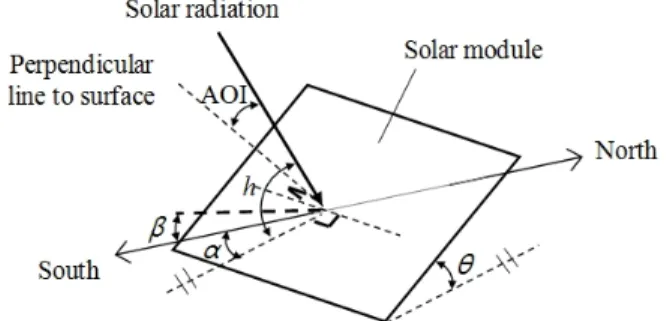
Although the intensity of the sunlight is constant, the short-circuit current of the solar module can change according to the AOI. As shown in Figure 1 and Eq. (1), the intensity of solar radiation arriving at the surface of the solar module is determined by the inclination angle and orientation of the solar module and the position of the sun. Moreover, the absorption and reflection from the glass cover of the solar module affect the intensity of the solar radiation reaching the solar cells in the solar module. The reflection rate of the glass cover significantly increases at an AOI of 40° (King, 1997). As a result, the intensity of the sunlight is proportional to the cosine of the AOI, and a slight error occurs owing to the glass cover.
The solar module is usually installed with a fixed tilt angle, for efficient power generation. However, in this study, the solar module was installed parallel to the
Figure 1. Angular relationships between the AOI and the surface of the solar module (h: solar altitude angle, α: surface azimuth angle, β: solar azimuth angle, θ: inclination angle of the surface).
ground because a solar module on a small IoT device is usually installed parallel to the body as this can reduce ambiguities that can result from other factors such as the reflection of sunlight or installation direction. When the solar module is installed parallel to the ground (θ = 0° and α = 0°), the solar altitude angle is 90° - AOI.
The AOI may be calculated from the solar altitude angle (h), the inclined angle of the surface (θ), the surface azimuth angle (α), and the solar azimuth angle (β) as follows:
cos sin·cos cos·sin·cos (1)
Air mass
The solar cell provides different responses based on different light spectra. For example, a mono-crystal Si exhibits good responsiveness at a wavelength of 900 nm, but poor responsiveness under 300 nm or over 1200 nm. As the sunlight passes through the atmosphere, the light is scattered and absorbed by air molecules. Therefore, the spectrum of the sunlight reaching the solar module varies according to the length of the atmosphere through which the sunlight passes, and this phenomenon must be considered in estimating the solar radiation from the solar module. Because the air mass (AM) provides an index of the optical path length through the atmosphere, this was chosen as an independent variable. The AM was calculated using Eq. (2), as proposed by Kasten and Young (1989):
AM ≈
cos
(2)
where Zs is the solar zenith angle, which is the difference between 90° and the solar altitude angle (Zs = 90 –h).
Cloud cover
When the solar module is partially or fully shaded by clouds, the short-circuit current of the solar module sharply decreases. The cloud cover provides an index of the fraction of the sky covered by clouds, and has an inverse relationship with the solar radiation. It is a dimensionless parameter, and is published on the Internet by the Meteorological Administration. It was assumed that an IoT device could collect this information
from the Internet.
Some researchers have attempted to estimate the solar radiation using the cloud cover. Kasten and Czeplak (1980) described the relationship between the solar radiation and amount of cloud, and this is expressed by Eqs. (3) and (4).
(3)
sin (4)
where IG and IGC are the global radiation under cloudy and cloudless weather conditions, respectively, and α is the AOI. The constant values (A, B, C, and D) must be estimated from the amount of cloud and the solar position. In addition, Yoo et al. (2008) applied these relations to estimate the solar radiation for major cities in Korea, and demonstrated strong correlations.
Experimental setup and data acquisition
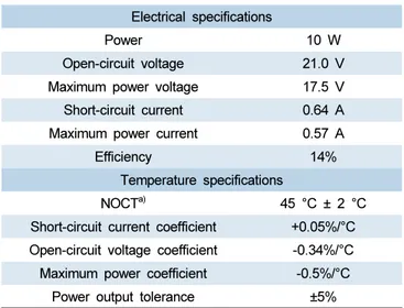
The solar module used for our experiment was connected in series with 36 mono-crystalline solar cell pieces without bypass diodes (TSM-10M, Shanghai Top Solar Green Energy, China). The maximum power was 10 W, and the open-circuit voltage was 2 1 V. The short- circuit current coefficient was 0.05%/°C and the maximum short-circuit current was 0.67 A under standard test conditions. Detailed specifications of the solar module are listed in Table 1.
Table 1. Specifications of the experimental solar module
Electrical specifications
Power 10 W
Open-circuit voltage 21.0 V Maximum power voltage 17.5 V Short-circuit current 0.64 A Maximum power current 0.57 A
Efficiency 14%
Temperature specifications
NOCTa) 45 °C ± 2 °C Short-circuit current coefficient +0.05%/°C Open-circuit voltage coefficient -0.34%/°C Maximum power coefficient -0.5%/°C
Power output tolerance ±5% a) Nominal operating cell temperature
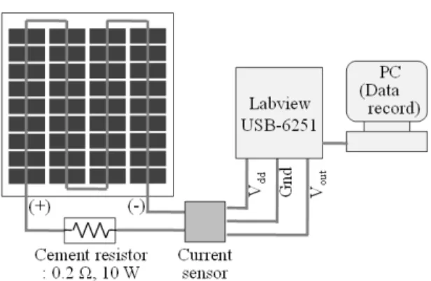
A Hall effect-based linear current sensor (WCS1702, Winson Semiconductor Corp., Taiwan) and a data acqui-sition device (USB-6251, National Instrument Corporation, USA) were utilized to measure the short-circuit current, as shown in Figure 2. The sensitivity of the current sensor was 1.0 mV·mA-1. The measured data was stored in a
MySQL (5.1.41., Oracle Corporation, USA) database. The short-circuit current was measured each second, and the average value per minute was employed. The ambient temperature and the reference solar radiation data were collected every minute using a PT-100 Ω sensor and a pyranometer (SYE-420M2007PM4, ShinYoung Electronics, Korea), respectively. The measurable range of the pyrano-meter was between 0 and 2000 W·m-2, and the error was
less than ±18 W·m-2 over a temperature range of −40°C to
80°C.
The experiment was conducted for approximately a year, from April 14 2011 to April 24 2012. There was some data loss for several days owing to weather problems, such as heavy snow or typhoons. All devices were installed on the roof of a one-story building at the Gyeonggi-do Agricultural Research and Extension Services, Republic of Korea (latitude: 37°13'21.27"N, longitude: 127°2'30.74"E), at a height of approximately 5.5 m from the ground. The solar module and
pyrano-meter were placed parallel to the ground. The hourly cloud cover data were collected from the Korean meteorological administration.
MLP learning for the model development
MLP was employed to create various models because it exhibits excellent potential for the prediction and classification of multi-variable data. In addition, it also achieved an accurate answer with a relatively lower computational complexity after the initial learning process. This represents a kind of black-box approach. This is usually employed to derive the results of a model rather than to confirm the mechanistic principles of the model.
The MLP method has frequently been employed to predict solar radiation since the mid-1990s. Elizondo et al. (1994) developed a neural network model that can predict daily solar radiation as a function of the daily maximum and minimum ambient temperatures, total daily precipitation, daily clear sky radiation, and day length. Reddy and Ranjan (2003) also developed an MLP model for estimating the mean daily and hourly values of the solar global radiation per month. In addition, there have been various trials conducted to estimate solar radiation using the MLP method (Sfetsos and Coonick, 2000; Dorvlo et al., 2002; Mellit et al., 2005).
In this study, the Fast Artificial Neural Network Library (FANN, version 2.1), which is an open source library and binds to various programming languages, was used to implement the MLP. The Python language was used to implement the learning and evaluation of the MLP using FANN. The input variables, algorithms, learning rate, activation function, number of hidden layers, and number of neurons should be chosen before MLP learning. The combinations of input variables for the MLP learning process were determined as shown in Table 2. Because the FANN library uses data ranging from 0 to 1, all input variables were standardized, and the output was
Figure 2. System configuration for the measurement and recording of the short-circuit current from the solar module.
Table 2. Combinations of input variables for MLP learning
Combination Input variables
I short-circuit current, ambient temperature II short-circuit current, ambient temperature, AOI
III short-circuit current, ambient temperature, AOI, air mass
IV short-circuit current, ambient temperature, AOI, air mass, cloud cover V short-circuit current, AOI, air mass, cloud cover
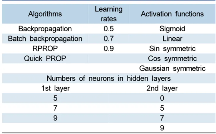
destandardized to obtain the estimated solar radiation. The configuration values chosen for the learning cycles are shown in Table 3. The algorithms consisted of standard backpropagation, batch backpropagation, RPROP (Igel and Hüsken, 2000) and Quick PROP (Fahlman, 1988). The standard backpropagation algorithm updates the weights after each training pattern, whereas batch backpropagation updates the weights after calculating the mean squared error (MSE) for the whole training set. The RPROP and Quick PROPs algorithms are advanced batch backpropagation algorithms described by Igel and Hüsken (2000) and Fahlman (1988), respectively. The learning rates, which affect the learning speed, were chosen arbitrarily as 0.5, 0.7, and 0.9. Five activation functions, which convert the given inputs to an output, were employed. The sigmoid function is the most frequently used activation function. The linear function requires less computing power. The Gaussian symmetric, sin symmetric, and cos symmetric functions were also utilized. One or two hidden layers were used because Negnevitsky (2004) explained that commercial MLPs incorporate three or sometimes four layers. When the number of neurons in the second hidden layer was zero, a second hidden layer was not utilized. Each layer could use different activation functions.
The total number of combinations for the MLP learning process was 14,400. Each learning cycle was repeated three times with random data, maintaining the same configuration. The data were divided into three groups: training, validation, and testing. First, 50 days of data were randomly chosen to test the developed models. Seventy percent of the remaining data were used for training, and the remainder were assigned for validation to check for overfitting.
The MSE is an indicator of the performance evaluation of the model (Eq. (5)). A smaller MSE indicates better performance because the backpropagation training algorithm aims to minimize this. The difference between the MSEs for training and validation was used to judge overlearning.
MSE ∑i (5)
where n is the number of data points for the training dataset, and sMSR and sESR are the standardized measured and estimated solar radiation, respectively.
Evaluation method
Various indices have been considered to evaluate the MLP model. Elizondo et al. (1994) utilized the coefficient of determination (R2 value) for evaluation. Reddy and
Ranjan (2003) used the maximum absolute error, mean absolute relative deviations, and percentage relative deviation to compare MLP models for the estimation of solar radiation with other correlation models. However, most researchers have employed the root-mean-squared error (RMSE) for evaluation (Sfetsos and Coonick, 2000; Dorvlo et al., 2002; Elminir et al., 2005). The daily RMSE was chosen as an evaluation index in this study.
The daily RMSE is defined as
RM SE
∑ (6)
where n is the number of data points on a day, and MSR and ESR are the measured and estimated solar radiation, respectively.
Results and Discussion
Characteristics of solar radiation and
short-circuit current
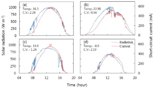
The short-circuit current is the most important variable in estimating solar radiation. Therefore, the short-circuit current and solar radiation were compared. One sunny day to represent each season was chosen because sunny days exhibited the full range of solar radiation (Fig. 3). The daily mean cloud cover of each day was between 1 and 3, and the average temperatures were
Table 3. Configuration values for MLP learning
Algorithms Learning
rates Activation functions Backpropagation 0.5 Sigmoid Batch backpropagation 0.7 Linear
RPROP 0.9 Sin symmetric Quick PROP Cos symmetric
Gaussian symmetric Numbers of neurons in hidden layers
1st layer 2nd layer
5 0
7 5
9 7
characteristic of each season. Figure 3 is presented such that 1200 W·m-2 of solar radiation was equivalent in scale
to 700 mA of short-circuit current. As shown in Figure 3, the short-circuit current varied along with solar radiation. However, the details of these changes were different.
First, the patterns of the solar radiation and short- circuit current were rather different. The solar radiation exhibited bilateral symmetry, whereas the short-circuit current was biased toward the later times of the day. In the morning, the ambient temperature was relatively low, and this might have caused a lower short-circuit current. Second, the amplitude of solar radiation was greater than that of the short-circuit current. As shown in Figure 3(a), solar radiation fluctuated around 8 am, but the short-circuit current did not. Because the maximum solar radiation in summer (Fig. 3(b)) was higher than in the other seasons, the tendency of the short-circuit current not to follow the changes in solar radiation became stronger. Overall, increases in solar radiation occurred prior to increases in the short-circuit current, and the increases and decreases of the short-circuit current were sharper than those of solar radiation.
To collect the correct short-circuit current, the solar module should be installed parallel to the ground. Although this decreases the efficiency of the solar module, it can reduce ambiguities that may result from the reflection of sunlight. The total radiation incident on the tilted solar module consists of three components: direct radiation, diffuse radiation, and radiation reflected
from the ground. The latter two components could induce increased errors in the estimation of solar radiation.
Results of MLP learning
The MSEs of the best MLP model were 0.0016 and 0.0022 for the training and validation datasets, respectively. Because the difference between the MSEs was under 1 W·m-2, the overfitting due to overlearning
was not severe. The desired MSE was set to 0.0015 for early stopping. However, none of the developed models achieved an MSE under 0.0015.
The RMSE of each learning cycle and the average over three repetitions were calculated. The average of RMSE of the best ANN model was 48.13 W·m-2. This result is better
than that of the regression model, for which the RMSE was 66.67 W·m-2 (Kim et al., 2012). Table 4 shows the
configuration of the best MLP model.
The best model for estimating solar radiation was applied for the days chosen in Figure 3, and the MSR and ESR were compared, as shown in Figure 4. The difference
Figure 3. Comparison of solar radiation and short-circuit current on (a) April 17, (b) June 20, and (c) October 1 2011 and (d) January 6 2012. Temp. and C.V. denote the daily mean ambient temperature (°C) and cloud cover (overcast=10) during sunlight hours.
Table 4. Configuration of the best MLP model
Combination of input variables
Learning
rate Algorithm IV 0.7 Batch backpropagation Number of neurons and activation function in hidden layer
1st layer 2nd layer 5, cos symmetric 9, sigmoid
between the ESR and MSR was largely reduced compared with the difference between the short-circuit current and MSR. The discrepancy between the increase in solar radiation and the increase in the short-circuit current almost disappeared. The daily RMSEs were evaluated as 45.75, 40.22, 67.50, and 26.72 W·m-2 on April 17, June 20,
and October 1 2011 and January 6 2012, respectively.
Accuracy analysis based on the RMSE
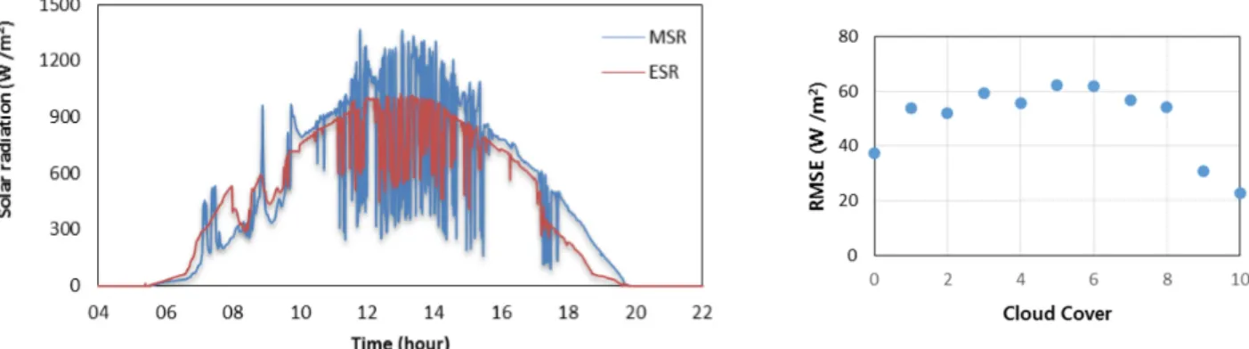
To determine the main causes of the errors, the daily variations in the MSR and ESR were examined. Figure 5 illustrates the daily variations in the MSR and ESR on July 19 2011, when the daily RMSE was 172.65 W·m-2, which
was the worst RMSE value of the model. As shown in Figure 5, there were many sudden variations in the MSR, and the ESR could not follow those changes.
Figure 6 illustrates the relationship between the RMSE
and cloud cover. The cloud cover provides an index of the fraction of the sky covered by clouds, with values of 0 and 10 representing a very sunny day and very cloudy day, respectively. The probability of fluctuations in solar radiation is lower on extremely sunny or very cloudy days. Therefore, the RMSE is lower for cloud cover values of 0, 9, and 10.
The main reason for this phenomenon lies the difference between covered areas that receive sunlight. The covered area of a pyranometer was significantly smaller than that of a solar module. If there are some variations in solar radiation over an area that is relatively small compared to a solar module but sufficiently wide to cover a pyranometer, this affects the measurement of the pyranometer but a solar module does not detect the difference. This is an inherent limitation of employing a solar module to measure solar radiation. Although the
Figure 4. Comparison of the measured and estimated solar radiation on (a) April 17, (b) June 20, and (c) October 1 2011 and (d) January 6 2012.
Figure 5. The worst daily RMSE on July 19, 2011, with sudden changes in solar radiation.
developed model exhibits good results, it does not completely overcome the limitation.
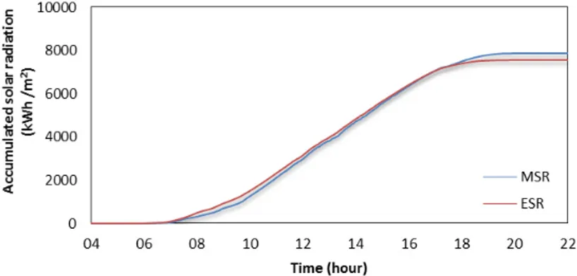
Accumulated solar radiation
The accumulated solar radiation, which is an important factor for agricultural use, has been employed to develop a plant growth model, estimate yields, or decide harvest times (Seshu and Cady, 1983; Roh and Lee, 1996; Linker and Seginer, 2003; Rosales et al., 2006). Although the developed model did not perform well in estimating sudden changes in solar radiation, the accumulated solar radiation was estimated reasonably accurately. Figure 7 illustrates the accumulated solar radiation on July 19 2011 depicted in Figure 5. On that day, the ESR did not follow the changes of the MSR. However, the accumulated solar radiations were 7.88 and 7.56 kWh·m-2 for the MSR and ESR, respectively, and
the estimation error of the model for the accumulated solar radiation was calculated as 4.06%.
This result represents a reasonable improvement compared to other models. Dorvlo et al. (2002) reported that the minimum RMSEs of the RBF and MLP were 230.74 Wh·m-2 and 280.78 Wh·m-2, respectively.
Furthermore, the RMSE of Elizondo et al. (1994)’s model varied from 811.76 to 1,011.92 Wh·m-2. The minimum
RMSE of the developed model was only 0.24 Wh·m-2, and
the average RMSE was 239.50 Wh·m-2. Thus, the
developed model exhibited superior results. It could be useful to estimate the accumulated solar radiation even on the days when solar radiation fluctuates.
Conclusions
The short-circuit current of a solar cell is known to be
proportional to solar radiation. This study was conducted to develop an MLP model to calculate solar radiation using the short-circuit current of a solar cell. The average RMSE for the best MLP model was evaluated as 48.13 W·m-2. The accuracy of this model was reduced on days
when solar radiation frequently varied, but the accumulated solar radiation was reasonably accurate. The average RMSE of the daily accumulated solar radiation was evaluated as 239.50 Wh·m-2.
Measuring solar radiation using an MLP model and solar module has some advantages. Although it requires time to collect the data and train the model, it only requires a small amount of computing power and time to estimate solar radiation using the trained model. The learning process could be accomplished using a high-powered computer, and the trained model could be applied on a small IoT device or embedded system. The second advantage lies in the simplicity of model replacement. An MLP model could be independently developed. If a new model is developed, then it is easy to replace the old model file with the new one. Finally, this method has an economic advantage. If an IoT device employs a solar module as a power source, then it is only necessary to add a current sensor. However, the price of a photodiode-type pyranometer is over $200, and the thermopile type is even more expensive. Based on these advantages, the developed model has potential for use in agricultural applications.
Conflict of Interest
The authors have no conflicting financial or other interests.
Acknowledgement
This work was supported by the Korea Institute of Planning and Evaluation for Technology in Food, Agriculture and Forestry (IPET) through the Advanced Production Technology Development Program, funded by Ministry of Agriculture, Food and Rural Affairs (MAFRA) (316077-03) and (117107-01)
References
Atzori, L., A. Iera and G. Morabito. 2010. The Internet of things: A survey. Computer Networks 54(15): 2787-2805. https://doi.org/10.1016/j.comnet.2010.05.010 Bowman, G.E., 1970. The transmission of diffuse light by
a sloping roof. Journal of Agricultural Engineering Research 15(2): 100-105.
https://doi.org/10.1016/0021-8634(70)90081-8 Cabrera, F. J., A. Baille, J. C. López, M. M. González-Real and
J. Pérez-Parra. 2009. Effects of cover diffusive properties on the components of greenhouse solar radiation. Biosystems Engineering 103(3): 344-356.
https://doi.org/10.1016/j.biosystemseng.2009.03.008 Dorvlo, A. S. S., J. A. Jervase and A. Al-Lawati. 2002. Solar
radiation estimation using artificial neural networks. Applied Energy 71(4): 307-319.
https://doi.org/10.1016/S0306-2619(02)00016-8 Elizondo, D., G. Hoogenboom and R. W. McClendon. 1994.
Development of a neural network model to predict daily solar radiation. Agricultural and Forest Meteorology 71(1-2): 115-132.
https://doi.org/10.1016/0168-1923(94)90103-1 Elminir, H. K., F. F. Areed and T. S. Elsayed. 2005.
Estimation of solar radiation components incident on Helwan site using neural networks. Solar Energy 79(3): 270-279.
https://doi.org/10.1016/j.solener.2004.11.006 Fahlman, S. E., 1988. An empirical study of learning speed
in back-propagation networks.
Huang, Y., L. Wu and J. Zhu. 2 010. Research of fuzzy control system about greenhouse supplement light lamps based on single-chip microcomputer. In: 2010 8th World Congress on Intelligent Control and Automation,
Paper No. 11511221. Jian, China: July 2010 https://doi.org/10.1109/WCICA.2010.5555032 Igel, C. and M. Hüsken. 2000. Improving the Rprop
learning algorithm. In: Proceedings of the Second ICSC International Symposium on Neural Computation (NC 2000), Berlin, Germany: May 2000.
Kaloxylos, A., R. Eigenmann, F. Teye, Z. Politopoulou, S. Wolfert, C. Shrank, M. Dillinger, I. Lampropoulou, E. Antoniou, L. Pesonen, H. Nicole, F. Thomas, N. Alonistioti and G. Kormentzas. 2012. Farm management systems and the future internet era. Computers and Electronics in Agriculture 89: 130-144.
https://doi.org/10.1016/j.compag.2012.09.002 Kasten, F. and G. Czeplak, 1980. Solar and terrestrial
radiation dependent on the amount and type of cloud. Solar Energy 24(2): 177-189.
https://doi.org/10.1016/0038-092X(80)90391-6 Kasten, F. and A. T. Young. 1989. Revised optical air mass
tables and approximation formula. Applied Optics 28(22): 4735-4738.
https://doi.org/10.1364/AO.28.004735
Kerr, J. P., G. W. Thurtell and C. B. Tanner. 1967. An Integrating pyranometer for climatological observer stations and mesoscale networks. Journal of Applied Meteorology 6(4): 688-694.
https://doi.org/10.1175/1520-0450(1967)006<0688:AIPFCO>2.0.CO;2 Kim, J. Y., S.-H. Yang, C. Lee, Y.-J. Kim, H.-J. Kim, S. I. Cho and
J. -Y. Rhee. 2012. Modeling of solar radiation using silicon solar module. Journal of Biosystems Engineering 37(1): 11-18.
https://doi.org/10.5307/JBE.2012.37.1.011
Kim, Y., R. G. Evans and W. M. Iversen. 2008. Remote sensing and control of an irrigation system using a distributed wireless sensor network. IEEE Transactions on Instrumentation and Measurement 57(7): 1379-1387. https://doi.org/10.1109/TIM.2008.917198
Kim, Y. H. and S. G. Lee. 1998. Analysis of the trans-missiviies of direct and diffuse solar radiation in multispan glasshouse. Journal of Biosystems Engineering 23(5): 439-444 (In Korean, with English abstract). King, D. L., 1997. Photovoltaic module and array
performance characterization methods for all system operating conditions. In: Proceeding of National Renewable Energy Laboratory (NREL) and Sandia National Laboratories (SNL) Photovoltaics Program Review Meeting, Lakewood, New York, USA: November 1996. King, D. L., W. E. Boyson and J. A. Kratochvil. 2004.
Photovoltaic array performance model. SAND 2004-3535. Albuquerque, New Mexico, California, USA: Sandia National Laboratories.
King, D. L. and D. R. Myers. 1997. Silicon-photodiode pyranometers: operational characteristics, historical experiences, and new calibration procedures. In: 26th Photovoltaic Specialists Conference, Paper No. 5900317. Anaheim, California, USA: Spetember 1997.
Klaring, H.-P., C. Hauschild, A. Heißner and B. Bar-Yosef. 2007. Model-based control of CO2 concentration in
greenhouses at ambient levels increases cucumber yield. Agricultural and Forest Meteorology 143(3-4): 208-216.
https://doi.org/10.1016/j.agrformet.2006.12.002 Linker, R. and I. Seginer. 2003. Water stress detection in a
greenhouse by a step change of ventilation. Biosystems Engineering 84(1): 79-89.
https://doi.org/10.1016/S1537-5110(02)00219-2 Malik, A. Q. and S. J. B. H. Damit. 2003. Outdoor testing of
single crystal silicon solar cells. Renewable Energy 28(9): 1433-1445.
https://doi.org/10.1016/S0960-1481(02)00255-0 Mellit, A., M. Menghanem and M. Bendekhis. 2005.
Artificial neural network model for prediction solar radiation data: application for sizing stand-alone photovoltaic power system, In: Power Engineering Society General Meeting, pp. 40-44, San Francisco, CA, USA: June, 2005.
Nash, E., P. Korduan and R. Bill. 2009. Applications of open geospatial web services in precision agriculture: a review. Precision Agriculture 10: 546-560.
https://doi.org/10.1007/s11119-009-9134-0 Negnevitsky, M., 2004. Artificial Intelligence: A Guide to
Intelligent Systems, 2nd ed, England: Boston.
Parretta, A., A. Sarno and L. R. M. Vicari. 1998. Effects of solar irradiation conditions on the outdoor performance of photovoltaic modules. Optics Communications 153(1-3): 153-163.
https://doi.org/10.1016/S0030-4018(98)00192-8 Reddy, K. S. and M. Ranjan. 2003. Solar resource estimation
using artificial neural networks and comparison with other correlation models. Energy Conversion and Management 44(15): 2519-2530.
https://doi.org/10.1016/S0196-8904(03)00009-8 Roh, M. Y. and Y. B. Lee. 1996. Control of amount and
frequency of irrigation according to integrated solar radiation in cucumber substrate culture.
Inter-national Symposium on Plant Production in Closed Ecosystems 440: 332-337.
https://doi.org/10.17660/ActaHortic.1996.440.58 Rosales, M. A., J. M. Ruiz, J. Hernández, T. Soriano, N.
Castilla and L. Romero. 2006. Antioxidant content and ascorbate metabolism in cherry tomato exocarp in relation to temperature and solar radiation. Journal of the Science of Food and Agriculture 86(10): 1545-1551.
https://doi.org/10.1002/jsfa.2546
Seshu, D. V. and F. B. Cady. 1983. Response of rice to solar radiation and temperature estimated from inter-national yield trials. Crop Science 24(4): 649-654. https://doi.org/10.2135/cropsci1984.0011183X002400040006x Sfetsos, A. and A. H. Coonick. 2000. Univariate and
multivariate forecasting of hourly solar radiation with artificial intelligence techniques. Solar Energy 68(2): 169-178.
https://doi.org/10.1016/S0038-092X(99)00064-X Sun, Y., L. Li, P. Schulze Lammers, Q. Zeng, J. Lin and H.
Schumann. 2009. A solar-powered wireless cell for dynamically monitoring soil water content. Computers and Electronics in Agriculture 69(1): 19-23.
https://doi.org/10.1016/j.compag.2009.06.009 Vellidis, G., M. Tucker, C. Perry, C. Kvien and C. Bednarz.
2008. A real-time wireless smart sensor array for scheduling irrigation. Computers and Electronics in Agriculture 61(1): 44-50.
https://doi.org/10.1016/j.compag.2007.05.009 Wang, N., N. Zhang and M. Wang. 2006. Wireless sensors
in agriculture and food industry—Recent development and future perspective. Computers and Electronics in Agriculture 50(1): 1-14.
https://doi.org/10.1016/j.compag.2005.09.003 Whillier, A., 1964. A Simple, accurate, cheap integrating
instrument for measuring solar radiation. Solar Energy 8(4): 134-136.
https://doi.org/10.1016/0038-092X(64)90075-1 Yoo, H.-C., K.-H. Lee and S.-H. Park. 2008. Analysis of data
and calculation of global solar radiation based on cloud data for major cities in korea. Journal of the Korean Solar Energy Society 28(4): 17-24 (In Korean, with English abstract)