Explicit Matrix Expressions of Progressive Iterative Approximation
Jie Chen1,2 and Guo-Jin Wang*1,2
1Department of Mathematics, Zhejiang University, Hangzhou 310027, China 2State Key Laboratory of CAD&CG, Zhejiang University, Hangzhou 310027, China
Abstract− Just by adjusting the control points iteratively, progressive iterative approximation (PIA) presents an intuitive and straightforward scheme such that the resulting limit curve (surface) can interpolate the original data points. In order to obtain more flexibility, adjusting only a subset of the control points, a new method called local progressive iterative approximation (LPIA) has also been proposed. But to this day, there are two problems about PIA and LPIA: (1) Only an approximation process is discussed, but the accurate convergence curves (surfaces) are not given. (2) In order to obtain an interpolating curve (surface) with high accuracy, recursion computations are needed time after time, which result in a large workload. To overcome these limitations, this paper gives an explicit matrix expression of the control points of the limit curve (surface) by the PIA or LPIA method, and proves that the column vector consisting of the control points of the PIA’s limit curve (or surface) can be obtained by multiplying the column vector consisting of the original data points on the left by the inverse matrix of the collocation matrix (or the Kronecker product of the collocation matrices in two direction) of the blending basis at the parametric values chosen by the original data points. Analogously, the control points of the LPIA’s limit curve (or surface) can also be calculated by one-step. Furthermore, the G1 joining conditions between two adjacent limit curves obtained from two neighboring data points sets are derived. Finally, a simple LPIA method is given to make the given tangential conditions at the endpoints can be satisfied by the limit curve.
Keywords: Explicit expression, Progressive iterative approximation, Local progressive iterative approximation, Limit control polygon, G1 joining
1. Introduction
In Computer Aided Geometric Design (CAGD), to fit or approximate the data points by using polynomial parametric curve (surface) is an important and basic project. Given a sequence of data points, in order to get a proper parametric curve (surface) which interpolates the original data points, a classical and effective method is called least-square method. In this method, the approximation curve (surface) can be derived by minimizing the least-square error. Recently, a new method called progressive iterative approximation (PIA) which can address the above project has been researched by many scholars (Lin et al., 2004, 2005; Delgado et al., 2007; Cheng et al., 2009; Lin, 2010; Lu, 2010; Chen et al., 2011). By adjusting the control points of a blending curve or patch iteratively, a sequence of curves or patches is generated progressively. With the increase of the iterative time, the distance between the original data points and the blending parametric curves or patches becomes more and more close, finally the limit curve (surface) can interpolate the original data points.
In (Ando, 1987), a type of totally positive matrices and their properties were discussed, this provided partial theoretic base of the research of the PIA property. In (Qi et al., 1975) and (de Boor, 1979), the PIA property for the uniform cubic B-spline basis was opened out, respectively. Later, in (Lin et al., 2004), this result was extended to the non-uniform cubic B-spline basis and the non-uniform bicubic tensor product B-spline surfaces; in (Lin et al., 2005), it was proved that both the curve and tensor product surface generated by the normalized totally positive (NTP) basis (Karlin, 1968) satisfied the PIA property. In (Delgado and Peña, 2007), the convergence rates of the different NTP basis were compared, and it was shown that the normalized B-basis satisfied the PIA property with the fastest convergence rates. In order to improve the iteration convergence rates, Lu (2010) introduced a new method of weighted PIA and gave a way to choose the optimal value of the weight. Cheng et al. (2009) constructed the loop subdivision surface based progressive interpola-tion. Furthermore, different from the previous method, Lin (2010) proposed an idea of local PIA which approximated only a chosen subset of the initial control points, not all of them, so it was more flexible. Chen and Wang (2011) extended the PIA property of the univariate NTP bases to the bivariate Bernstein basis over a triangle domain for constructing triangular Bézier surfaces. However, the limit location of the PIA model cannot be calculated accurately, and if the higher *Corresponding author:
Tel: +86-0571-8795-1609 Fax: +86-0571-8795-1358 E-mail: wanggj@zju.edu.cn
accuracy is requested by users, the time-consuming iterative calculation must be needed. This severely affects the efficiency in reverse engineering applica-tions by the PIA method. As for the method of fitting data points based on the subdivision technique, Suzuki et al. (1999) have pointed out that, “The basic idea is to use the subdivision limit position (SLP) to adapt the control mesh of the subdivision surface to the data points….It does…fail to capture local characteristics of data points. Consequently, the proposed method is not suitable for generating a surface that precisely inter-polates the data points.” On the other hand, Generating subdivision surface always needs some subdivision steps for a net which is a considerable time consuming process. To overcome these shortcomings, this paper gives an explicit expression of the control points of the limit curve (surface) by the PIA or LPIA method. Its strongpoint consists in that, firstly the interpolation for data points by our limit curve (surface) is precise absolutely, and secondly the evaluation process is direct and rapid because it needs only a matrix multiplication by using the explicit expression. In a word, both the computational accuracy and efficiency could be reached optimal simultaneity. Moreover, the G1 continuous con-dition between two limit curves generated by two adjacent data sets respectively using the PIA method is derived. An application of this method is that the interpolation problem of the scattered data points can be converted to the piecewise joining of local interpola-tions, at the same time the G1 continuity can be satisfied between all the adjacent curves. At last, a simple method is discussed to show that any given tangential condition at the endpoints can be satisfied by the limit curve using the LPIA method.
2. Explicit Expressions of the Control Points
of the Limit Curve (Surface)
2.1 In the case of PIA method
Given a sequence of points , each point Pi is
assigned to a parameter value ti, i = 0, 1, …, n. Let
(B0(t), B1(t), …, Bn(t)) be a blending basis, that is, each
basis function is nonnegative and satisfied the
expression . Then we obtain an initial curve
(1) For every control point Pi, letting an adjusting vector
(2) and new data point
(3) we can get the second curve
(4) Similarly, we can get the curve Ck+1(t) after the (k+1)-th iteration
(5) where
; (6)
If , we call that the initial
curve C0(t) has the PIA property. In the iterative process, for the adjusting vectors set
(7) we obtain the iterative format ∆k+1= (I − B)∆k, where I is the identity matrix, and
(8) is the collocation matrix of the blending basis (B0(t),
B1(t), …, Bn(t)) at the parametric values .
It is obvious that if the spectral radius of the matrix I− B is less than 1, i.e., ρ(I − B) < 1, then .
The control points after k + 1 iterations can be expressed as
i = 0, 1, …, n; k = 0, 1, …. Letting
, (9)
,
we rewrite the above formulas in matrix form: (10) Since B is a nonsingular matrix,
As ρ(I − B) < 1, then (11) Pi { }i=0n Bit() i=0 n
∑
=1 C0 t() Σ= i=0n PiBi t() ∆i0=Pi–C0( )ti i 0 1 … n= , , , Pi1=Pi0+∆i0 i 0 1 … n= , , , C1 t() Σ= i=0n Pi1Bi t() Ck 1+ t() Σ= i=0n Pik 1+ Bi t() ∆ik=Pi–Ck( )ti i 0 1 … n= , , , Pik 1+ =Pik+∆ik i 0 1 … n= , , , Ck( )ti k ∞lim→ Pi 0 = i 0 1 … n= , , , ∆k=[∆0k, , ,∆1k… ∆kn]T (k 0 1 …= , , ) B B0, ,… Bn t0, ,… tn ⎝ ⎠ ⎛ ⎞: B( j( )ti) i=0 … n, , j=0 … n, , = ti { }i=0n Ck( )ti k ∞lim→ Pi 0 = Pik 1+ =Pik+∆ik=Pik+Pi–Ck( )ti =Pi+Pik–Σnj=0PjkBj( )ti Pk 1+ =[P0k 1+,P1k 1+, ,… Pnk 1+]T Pk=[P0k, , ,P1k… Pnk]T P P=[ 0, , ,P1 … Pn]T Pk 1+ –P=(I B– )Pk Pk 1+ –B–1P=(I B– ) P( k–B–1P) I B=( – )2(Pk 1– –B–1P) =…=(I B– )k(P B– –1P) Pk 1+ k ∞lim→ B 1 – P =This means that the control points of the limit curve which interpolates the original data points are B-1P. Thus, the column vector consisting of the control
points of the PIA’s limit curve can be obtained by multiplying the column vector P consisting of on the left by the inverse matrix of the collocation
matrix , generating from the blending
basis with the parametric values , which
are chosen by . It is evident that the
computa-tional process is simple and direct and the result is accurate.
Similarly, we can discuss the case of surfaces. Given
a sequence of points , each point Pi,j is
assigned to a pair of parameter values (ui, vj), i = 0,
1, …,m, j = 0, 1, …, n, where
, .
Similar with the case of curves, we can obtain an initial surface
(12) and a sequence of surfaces
(13) where
, , i = 0, 1, …, m; j = 0, 1, …, n; k = 0, 1, …. (14)
If , i = 0, 1, …, m, j = 0, 1, …, n, we
call that the initial surface S0(u, v) has the PIA property. Suppose that
k = 0, 1, … (15)
the iterative format for ∆k is ∆k+1= (I − B)∆k, where I is the identity matrix, and B is the Kronecker product of two collocation matrices B1 and B2, that is B = B1⊗B2,
here
, (16)
It is obvious that if the spectral radius of the matrix I− B is less than 1, i.e., ρ(I − B) < 1, then . The control points after k+1 iterations can be expressed as (17) i = 0, 1, …, m; j = 0, 1, …, n; k = 0, 1, …. Letting Pk+1= [ , , …, , , …, , …, , …, ]T (18) (19) (20) We rewrite the above formulas in matrix form:
(21) Noting that B is a nonsingular matrix, so
As ρ(I − B) < 1, then
(22) This indicate that the control points of the limit surface which interpolates the original data points are B-1P. Thus, the column vector consisting of the control points of the PIA’s limit surface can be computed straight by multiplying the column vector P
consisting of on the left by the inverse
matrix of the Kronecker product B = B1⊗B2, where B1,
B2 are two collocation matrices of the blending basis
and at the parametric values
, , respectively, corresponding to .
2.2 In the case of LPIA method
In order to obtain more flexibility, Lin (2010) presented a new method called local progressive iterative appro-ximation. This method only approximated a subset of the initial points, not all of them. The main idea and skill is only adjusted a subset of the control points in the iterative processes. And the shape of the parametric curves (surfaces) can be adjusted locally.
Given a set of the points , we suppose only
the points are adjusted, and the other
po-ints, the remain unchanged. Different from
global PIA method, the new control points at each iterative step are given by
(23) l∈{j0, j1,…,jJ}, k=0,1,…, h∈{i0, i1,…,iI}, k=0,1,…, Pi { }i=0n Pi { }i=0n B B=( j( )ti )i=0 … nj=0 … n, ,, , Bi { }i=0n { }ti i=0n Pi { }i=0n Pi j, { }i=0 j=0m n u0< < <u1 … um v0< < <v1 … vn S0(u v, ) Pi j0, Bi( )Bu j( )v j=0 n
∑
i=0 m∑
= Sk(u v, ) Pi j,kBi( )Bu j( ) k=0,1,…v j=0 n∑
i=0 m∑
= ⎩ ⎭ ⎨ ⎬ ⎧ ⎫ Pi j0, =Pi j, { }i=0 j=0m n Pi jk 1,+ =Pi j,k+∆i jk, ∆i jk,=Pi j,–Sk(ui,vj) Sk(u v, ) k ∞lim→ Pi j, 0 = ∆k=[∆0 0k, ,∆0 1k, , ,… ∆0 nk,,∆1 0k,, ,… ∆l1 n,, ,… ∆m 1k, , ,… ∆m nk, ]T B1=(Bj( )ui )i=0 … mj=0 … m, ,, , B2=(Bj( )vi )i=0 … nj=0 … n, ,, , Sk(u v, ) k ∞lim→ Pi j, 0 = Pi jk 1,+ =Pi jk,+∆i jk, =Pi jk,+Pi j, –Sk(ui,vj) =Pi j, +Pi j,k–Σl=0m Σh=0n Pl h,kBl( )Bui h( )vj P0 0k 1,+ P0 1k 1,+ P0 nk 1,+ P1 0k 1,+ P1 nk 1,+ Pm 1k 1+, Pm nk 1+, Pk=[P0 0k,,P0 1k,, ,… P0 nk,,P1 0k,, ,… P1 nk,, ,… Pm 1k, , ,… Pm nk, ]T P P=[ 0 0, ,P0 1, , ,… P0 n, ,P1 0,, ,… P1 n,, ,… Pm 1, , ,… Pm n, ]T Pk 1+ –P=(I B– )Pk Pk 1+ –B–1P=(I B– ) P( k–B–1P) I B=( – )2(Pk 1– –B–1P) =…= I B( – )k(P B– –1P) Pk 1+ k ∞lim→ B 1 – P = Pi j, { }i=0 j=0m n Pi j, { }i=0 j=0m n Bi( )u { }i=0m {Bj( )v }j=0n ui { }i=0m { }vj j=0n { }Pi j, i=0 j=0m n Pi { }i=0n i0th, , ,i1th… iIth j0th, , ,j1th… jJth Plk 1+ =Pl Plk 1+ Phk+∆hk Phk Ph PjkBj( )th j=0 n∑
– ⎝ ⎠ ⎜ ⎟ ⎛ ⎞ + = = ⎩ ⎪ ⎪ ⎨ ⎪ ⎪ ⎧Letting
(24) (25) (26) We rewrite the above formulas in matrix form as follows:
(27) where
(28)
(29)
here IJ+1 is the (J + 1) × (J + 1) identity matrix, 0 is
the (J + 1) × (J + 1) zero matrix. Note that B is a non-singular matrix, so B is also a nonsingular matrix, then
Since ρ (II+1− B2) < 1,
(30) So we find that the control points of the LPIA’s limit curve which interpolates the partial original data points
are B-1P.
Next we discuss the case of surfaces briefly. Given a
set of the points , we suppose only the
points with the subscripts {(i0, j0), (i1, j1), …, (iJ, jJ)} are
adjusted, and the other points with the subscripts {(k0,
l0), (k1, l1), …, (kJ, lJ)} remain unchanged. The new
con-trol points at each iterative step are given by
(31)
Letting
(32) (33) (34) We rewrite the above formulas in matrix form as
(35) where
(36)
(37)
(38)
here IJ+1 is the (J + 1)× (J + 1) identity matrix, 0 is
the (J + 1)× (J + 1) zero matrix. Noting that B is a non-singular matrix, so B is also a nonsingular matrix, then
Since ρ (II+1− B2) < 1,
(39) It follows that the LPIA’s control points of the limit surface which interpolates the partial original data
points are B-1P.
2.3 Examples
Example 2.1 Consider the curve given by , t ∈ [0, 2π] Pk 1+ Pj0 k 1+ P j1 k 1+ … P jJ k 1+ P i0 k 1+ P i1 k 1+ … P iI k 1+ , , , , , , , [ ]T = Pk Pj0 k P j1 k … P jJ k P i0 k P i1 k … P iI k , , , , , , , [ ]T = P P[ j0, , , , , , ,Pj1… PjJ Pi0Pi1… PiI] T = Pk 1+ =P I+( n 1+ –B˜)Pk B˜ IJ 1+ 0 D1 B2 ⎝ ⎠ ⎛ ⎞ = B2 Bi0( )Bti0 i1( )…Bti0 iI( )ti0 Bi0( )Bti1 i1( )… Bti1 iI( )tiI … … … … Bi0( ) BtiI i1( ) … BtiI iI( )tiI = Pk 1+ –B˜–1P=(I B˜– ) P( k–B˜–1P) I B˜=( – )k 1+ (P B˜– –1P) = 0 0 D1 – II 1+ –B2 ⎝ ⎠ ⎛ ⎞k 1+ P B˜–1P – ( ) = 0 0 II 1+ –B2 ( )kD1 – (II 1+ –B2)k 1+ ⎝ ⎠ ⎜ ⎟ ⎛ ⎞ P B˜– –1P ( ) Pk 1+ k ∞lim→ B˜ 1 – P IJ 1+ 0 B2–1D1 – B2–1 ⎝ ⎠ ⎜ ⎟ ⎛ ⎞ P = = Pi { }i∈{i0, , ,i1… iI} Pi j, { }i=0 j=0m n Pl hk 1,+ =Pl h, l h, ( )∈{(k0,l0) k,( 1,l1) … k, ,( J,lJ)},k=0 1 …,, , Pl hk 1,+ Pl hk, +∆l hk, Pl hk, Pl h, Pi j,kBi( )Bul j( )vh j=0 n
∑
i=0 m∑
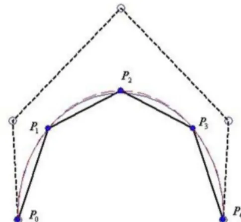
– ⎝ ⎠ ⎜ ⎟ ⎛ ⎞ + = = l h, ( )∈{(i0,j0) i,(1,j1) … i, ,(I,jI)},k=0 1 …,, , ⎩ ⎪ ⎪ ⎪ ⎨ ⎪ ⎪ ⎪ ⎧ Pk 1+ Pk0,l0 k 1+ P k1,l1 k 1+ … P kJ,lJ k 1+ … P i0,j0 k 1+ P i1,j1 k 1+ … P iI,jI k 1+ , , , , , , , , [ ]T = Pk Pk0,l0 k P k1,l1 k … P kJ,lJ k … P i0,j0 k P i1,j1 k … P iI,jI k , , , , , , , , [ ]T = P P[ k0,l0,Pk1,l1, ,… PkJ,lJ, ,… Pi0,j0,Pi1,j1, ,… PiI,jI] T = Pk 1+ =P I+( n 1+ –B˜)Pk B˜ IJ 1+ 0 D1 B2 ⎝ ⎠ ⎛ ⎞ = D1 Bk0( )Bui0 l0( )Bvj0 k1( )Bui0 l1( )…Bvj0 kJ( )Bui0 lJ( )vj0 Bk0( )Bui1 l0( )Bvj1 k1( )Bui1 l1( )…Bvj1 kJ( )Bui1 lJ( )vj1 … … … … Bk0( )BuiI l0( ) BvjI k1( )BuiI l1( ) … BvjI kJ( )BuiI lJ( )vjI I 1+ ( ) J 1×(+ ) = B2 Bi0( )Bui0 j0( )Bvj0 i1( )Bui0 j1( )…Bvj0 iI( )Bui0 jI( )vj0 Bi0( )Bui1 j0( )Bvj1 i1( )Bui1 j1( )…Bvj1 iI( )Bui1 jI( )vj1 … … … … Bi0( )BuiI j0( ) BvjI i1( )BuiI j1( ) … BvjI iI( )BuiI jI( )vjI I 1+ ( ) I 1×(+ ) = Pk 1+ –B˜–1P=(I B˜– ) P( k–B˜–1P) I B˜=( – )k 1+ (P B˜– –1P) = 0 0 D1 – II 1+ –B2 ⎝ ⎠ ⎛ ⎞k 1+ P B˜–1P – ( ) = 0 0 II 1+ –B2 ( )kD1 – (II 1+ –B2)k 1+ ⎝ ⎠ ⎜ ⎟ ⎛ ⎞ P B˜– –1P ( ) Pk 1+ k ∞lim→ B˜ 1 – P IJ 1+ 0 B2–1D1 – B2–1 ⎝ ⎠ ⎜ ⎟ ⎛ ⎞ P = = Pi j, { }( )i j,∈{(i0,j0) i,(1,j1) … i, ,(I,jI)} x t() y t(), ( )=(–cos t(),sint())A sequence of 5 points is sampled from the parameter curve
, ,
Letting be the control points, we can obtain
an initial Bézier curve of degree 4 as follows: , t ∈ [0, 1]
Where are the Bernstein basis
func-tions of degree 4. For convenience, we choose the
uniform parameters , the inverse matrix of
the collocation matrix B of the blending basis
is
(40)
Then the column vector consisting of the control points of the limit curve can be instantly calculated by multiplying the column vector P consisting of on the left by Eq. (40):
B-1P = ((-1,0), (-1.052,0.771), (0,1.639), (1.052,0.771),
(1,0))T
It is obvious that the result is absolutely accurate and the computational process is very fast because we need only a matrix multiplication and also Eq. (40) can be computed beforehand.
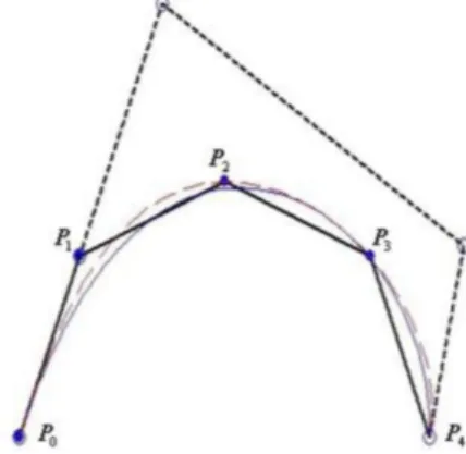
Fig. 2.1~2.3 illustrate the initial Bézier curve and the approximation curve after different iterations respec-tively by the PIA method. Fig. 2.4~2.6 illustrate the initial Bézier curve and the approximation curve
Example 2.2 A sequence of points are
given by {(-1, 0.8, 1), (0.1, 1, 1.2), (0.8, 0.6, 0.9), (-1.2,
0, 1.3), (0, 0, 1.5), (1, -0.2, 1), (-0.9, -0.8, 0.9), (0.2, -0.7, 1.2), (0.9, -0.6, 0.9)}, the corresponding initial bi-quad-ratic tensor product Bézier surface is
For convenience, we choose the uniform parameters , .
The Kronecker product B of two collocation matrices B1 and B2 is Pi { }i=04 Pi=(x s( ) y si , ( )i ) si=i π⋅---4 i 0 1 … 4= , , , Pi { }i=04 B0 t() PiBi t() i=0 4
∑
= Bit() 4 i ⎝ ⎠ ⎛ ⎞ 1 t( – )4 i–ti = ti=i/4 { }i=04 Bi t() { }i=04 B–1 1 0 0 0 0 1.083 – 4 –3 1.333 –0.25 0.722 –3.556 6.667 –3.556 0.722 0.25 – 1.333 –3 4 –1.083 0 0 0 0 1 ⎝ ⎠ ⎜ ⎟ ⎜ ⎟ ⎜ ⎟ ⎜ ⎟ ⎜ ⎟ ⎛ ⎞ = Pi { }i=04 Pi j, { }i=0 j=02 2 S0(u v, ) Pi j,Bi( )Bu j( )v j=0 2∑
i=0 2∑
= ui=i/2 { }i=02 {vj=j/2}j=02Fig. 2.1. Global approximation-initial Bézier curve.
Fig. 2.2. Global approximation-after the 1st iteration.
Fig. 2.3. Global approximation-after the 5th iteration.
The inverse matrix of B is
(41)
Then the column vector consisting of the control points of the limit surface can be directly obtained by
multiplying the column vector P consisting of
on the left by Eq. (41):
B-1P = {(-1,0.8,1), (0.3,1.3,1.45), (0.8,0.6,0.9), (-1.45,
0,1.6,5), (-0.15,-0.1,2.225), (1.15,-0.4,1.1), (0.9,-0.8,0.9), (0.4,-0.7,1.5), (0.9,-0.6,0.9)}
It is evident that the result is absolutely accurate and the computational process is very rapid because we need only a matrix multiplication and also Eq. (41) can be computed beforehand.
Fig. 2.7~2.9 illustrate the initial Bézier surface and the approximation surfaces after different iterations res-pectively by the PIA method. Fig. 2.10~2.12 illustrate the initial Bézier surface and the approximation sur-faces after different iterations respectively by the LPIA method (approximating P1,0 and P1,1 only). In each
figure, the original control points and the control points of the limit surfaces are marked by solid points and hollow points respectively. Moreover, the limit surfaces and the approximation surfaces after different iterations are illustrated by grid surfaces and solid surfaces res-pectively.
Example 2.3 In order to compare practical effects in reverse engineering between our method and subdivi-sion technique, using the same set of data points locating on a face, shown as in Fig. 2.13, the algorithm of this paper and Loop subdivision algorithm (Loop, 1987) have been implemented, and the final results can be shown as in Fig. 2.15 and Fig. 2.16, respectively. Also Fig. 2.14 can be given if we implement conven-tional PIA after the first iteration. It is obvious to see that the subdivision algorithm and conventional PIA failed to capture local characteristics of data points, but our method can interpolate the all original data points accurately.
3.
G
1joining between two adjacent limit curve
Given two adjacent sequences of points and
, where P0=Q0. Also denoting the Bernstein
basis functions of degree n and m by ( (t), (t), …,
1 0 0 0 0 0 0 0 0 1/4 1/2 1/4 0 0 0 0 0 0 0 0 1 0 0 0 0 0 0 1/4 0 0 1/2 0 0 1/4 0 0 1/16 1/8 1/16 1/8 1/4 1/8 1/16 1/8 1/16 0 0 1/4 0 0 1/2 0 0 1/4 0 0 0 0 0 0 1 0 0 0 0 0 0 0 0 1/4 1/2 1/4 0 0 0 0 0 0 0 0 1 ⎝ ⎠ ⎜ ⎟ ⎜ ⎟ ⎜ ⎟ ⎜ ⎟ ⎜ ⎟ ⎜ ⎟ ⎜ ⎟ ⎜ ⎟ ⎜ ⎟ ⎜ ⎟ ⎜ ⎟ ⎜ ⎟ ⎛ ⎞ 1 0 0 0 0 0 0 0 0 1/2 – 2 –1/2 0 0 0 0 0 0 0 0 1 0 0 0 0 0 0 1/2 – 0 0 2 0 0 –1/2 0 0 1/16 1/8 1/16 1/8 1/4 1/8 1/16 1/8 1/16 0 0 –1/2 0 0 2 0 0 –1/2 0 0 0 0 0 0 1 0 0 0 0 0 0 0 0 –1/2 2 –1/2 0 0 0 0 0 0 0 0 1 ⎝ ⎠ ⎜ ⎟ ⎜ ⎟ ⎜ ⎟ ⎜ ⎟ ⎜ ⎟ ⎜ ⎟ ⎜ ⎟ ⎜ ⎟ ⎜ ⎟ ⎜ ⎟ ⎜ ⎟ ⎜ ⎟ ⎛ ⎞ Pi j, { }i=0 j=02 2 Pi { }i=0n Qi { }i=0m B0n B1n
Fig. 2.5. Local approximation-after the 1st iteration.
Fig. 2.6. Local approximation-after the 5th iteration.
(t)) and respectively, we can interpolate these two original data points sets by the PIA method respectively. Suppose that the limit curve which interpolates is C1(t), satisfying C1(ti) =Pi,
i = 0, 1, …, n; the limit curve which interpolates
is C2(t), satisfying C2(τj) =Qj, j = 0, 1, …, m. We will
discuss the conditions of G1 joining between two adjacent limit curve C1(t) and C2(t).
Lemma 3.1 (Wang et al., 2001) Denote the Bernstein basis functions of degree n by ( (t), (t), …, (t)),
; given the control points , we can
obtain the initial Bézier curve as follows: Bnn (B0m t() B, m1 t() … B, , mm t()) Pi { }i=0n Qi { }i=0m B0n B1n Bnn t 0 1∈[ , ] { }Pi i=0n
Fig. 2.8. Global approximation-after the 1st iteration.
Fig. 2.9. Global approximation-after the 5th iteration.
Fig. 2.10. Local approximation-initial Bézier surface.
Fig. 2.11. Local approximation-after the 1st iteration.
Fig. 2.12. Local approximation-after the 5th iteration.
Fig. 2.13. The original mesh of a face.
Fig. 2.14. The resultant surface generated by PIA whose iteration level is 1, based on the original mesh of a face shown in Fig. 2.13.
; The 1st derivative of B(t) is
. Specially, the 1st derivatives at the endpoints of the curve are B'(0) = n(P1− P0), B'(1) = n(Pn− Pn-1).
Denote the collocation matrices of the Bernstein basis
functions , at the parameters
, by Bn and Bm, respectively. Letting P =
[P0, P1, …, Pn]T, Q = [Q0, Q1, …, Qm]T, we suppose G =
[G0, G1, …, Gn]T and H = [H0, H1, …, Hm]T are the
con-trol points of the limit curves C1(t) and C2(t)
respec-tively. Then the explicit expressions of the control points of these two limit curves are
,
The necessary and sufficient conditions of G1 joining C1(t) and C2(t) at the endpoint P0=Q0 are
Where l is an arbitrary real number. As C1(t0) =P0
=Q0=C2(τ0), the first condition of the above formula is
satisfied naturally.
For convenience, we take t0=τ0= 0. From Lemma
3.1, we know that the condition C'1(t0) =l·C'2(τ0) is
equivalent to
That is
(40)
Where is the element of the matrix in the
ith row and jth column.
Especially, if n = m, then the necessary and sufficient conditions of G1 joining C1(t) and C2(t) at the endpoint
P0=Q0 are
(41) Example 3.1 Consider the curve given by
, t ∈ [0, 2π]
A sequence of 5 points is sampled from the
parameter curve
, ,
The other curve is given by ,
A sequence of 5 points is sampled from the
parameter curve
, ,
Letting and be the control points of
two Bézier curves, respectively, we can obtain two initial Bézier curves of degree 4 respectively as follows:
, ,
Where are the Bernstein basis
func-tions of degree 4. For convenience, we choose the
uniform parameters .
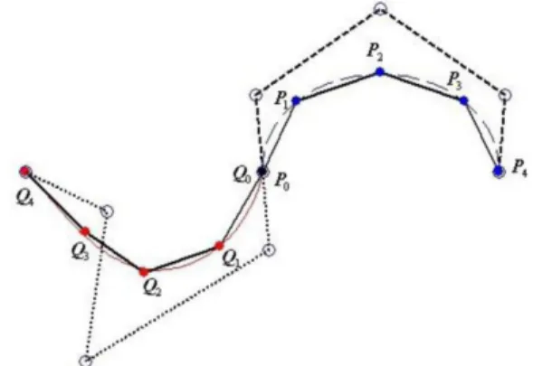
It is obvious that the G1 joining conditions of the two Bézier curves can be satisfied by the original control
points and . Fig. 3.1 shows the joining
effect of two limit curves. Fig. 3.2~3.3 are for the B t() PiBin t() i=0 n
∑
= B′ t() n (Pi 1+ –Pi)Bin 1– t() i=0 n 1–∑
= Bin t() { }i=0n {Bjm t()}j=0m ti { }i=0n { }τj j=0m G B= n–1P H B= m–1Q C1( ) Ct0 = 2( )τ0 C′1( ) l C′t0 = ⋅ 2( )τ0 ⎩ ⎨ ⎧ n G( 1–G0) lm H= ( 1–H0) n ((Bn–1)1k–(Bn–1)0k)Pk k=0 n∑
lm ((Bm–1)1k–(Bm–1)0k)Qk k=0 m∑
= Bn–1 ( )ij Bn–1 Bn–1 ( )1k–(Bn–1)0k ( ) P( k–lQk) k=1 n∑
=0 x t() y t(), ( ) 1=( –cos t(),sin t()) Pi { }i=04 Pi=(x s( ) y si , ( )i ) si=i π⋅---4 i 0 1 … 4= , , , x t() y t(), ( )=(cos t()–1,–sin t()) t 0 2π∈[ , ] Qi { }i=04 Qi=(x s( ) y si , ( )i ) si=i π⋅---4 i 0 1 … 4= , , , Pi { }i=04 { }Qi i=04 C10 t() PiBi t() i=0 4∑
= C20 t() QiBi t() i=0 4∑
= t 0 1∈[ , ] Bit() 4 i ⎝ ⎠ ⎛ ⎞ 1 t( – )4 i–ti = ti=i/4 { }i=04 Pi { }i=04 { }Qi i=04Fig. 2.15. The resultant surface generated by our method, based on the original mesh of a face shown in Fig. 2.13.
Fig. 2.16. The resultant mesh generated by Loop subdivision, based on the original mesh of a face shown in Fig. 2.13.
demonstration of the joining effect by fixing
and adjusting a part of . In each figure, the
original control points , and the control
points of the limit curves are marked by solid points and hollow points respectively. Moreover, the limit curves C1(t) and C2(t) are illustrated by solid lines and
dashed lines respectively.
4. The LPIA method with
tangential conditions at endpoints
In this section, we give a simple method, so that not only the original data points can be interpolated, but
also the given tangential conditions can be satisfied by the limit curve using the LPIA method.
Given a sequence of points , each point Pi is
assigned to a parameter value ti, i = 0, 1, …, n. Let (B0(t),
B1(t), …, Bn(t)) be a Bernstein basis of degree n, and
denote the limit Bézier curve interpolating the original points by C(t), satisfying C1(ti) =Pii = 0, 1, …,
n. Suppose that t0= 0, that is C1(t0) =P0.
From Lemma 3.1, it is obvious that the tangent direction at the endpoint of a Bézier curve is deter-mined by the control points P0 and P1. In order to make
the tangent direction at the endpoint P0 of the limit
curve C(t) is consistent with the vector α, that is C'(t0)
Pi { }i=04 Qi { }i=04 Pi { }i=04 { }Qi i=04 Pi { }i=0n Pi { }i=0n
Fig. 3.1. G1 joining of two limit curves.
Fig. 3.2. G1 joining of two limit curves (After adjusting Q 1, Q2).
Fig. 3.3. G1 joining of two limit curves (After adjusting Q 1, Q3).
Fig. 4.1. Tangential direction α = (-1, 2) at P0.
Fig. 4.2. Tangential direction α = (-1, 1) at P0.
□α, we add an auxiliary control point along the direction P0+kα (k > 0), which is denoted by P-1, and
extend the original data points to . Then at
each step of iteration process, the n + 1 control points are adjusted, the point remain unchanged, so the tangent direction of the limit curve is parallel to the vector α.
Example 4.1 Consider the curve given by , t ∈ [0, 2π]
A sequence of 5 points is sampled from the
parameter curve
, ,
Fig. 4.1~4.3 illustrate the approximation effects by the LPIA method with different tangential conditions at the endpoint P0. In each figure, the original control
points and the adding point are marked by
solid points and hollow-block point respectively. Moreover, the limit curves C(t) and the corresponding control points are illustrated by solid lines and hollow points respectively.
5. Conclusion
It is intuitive, stable and flexible to interpolate the data points by the PIA method. In order to obtain the limit curves (surfaces) rapidly, directly and accurately by recursive iterations, using the tool of collocation matrix, we get the explicit expressions of the control points of the limit curves (surfaces) by the PIA and the LPIA method. This result is effectual and simple, and the approximation errors can be ignored. Furthermore, based on this simple explicit expression, the G1 joining conditions between two adjacent limit curves are derived. This method can be extended to the G1 joining of multiple limit curves similarly. The convex-pre-serving conditions of the limit curves with constrained tangential conditions can be researched in future work.
Acknowledgements
This work was supported by the National Natural
Science Foundations of China under Grant No. 6107-0065 and No. 60933007.
References
[1] Ando T. 1987. Totally positive matrices. Linear Algebra Applications, 90, 165-219.
[2] Chen J. and Wang G. J. 2011. Progressive-iterative approximation for triangular Bézier surfaces. to appear in Computer-Aided Design.
[3] Cheng F. H., Fan F. T., Lai S. H., Huang C. L., Wang J. X., and Yong J. H. 2009. Loop subdivision surface based progressive interpolation. Journal of Computer Science and Technology, 24, 39-46.
[4] de Boor C. 1979. How does Agee’s smoothing method work? In: Proceedings of the 1979 Army Numerical Analysis and Computers Conference, ARO Report 79-3, Army Research Office, 299-302.
[5] Delgado J. and Peña J. M. 2007. Progressive iterative approximation and bases with the fastest convergence rates. Computer Aided Geometric Design, 24(1), 10-18. [6] Karlin S. 1968. Total positivity, Volumn I. Standford
University Press, Standord, C.A.
[7] Lin H. W. 2010. Local progressive-iterative approximation format for blending curves and patches. Computer Aided Geometric Design 27, 322-339.
[8] Lin H. W., Bao H. J. and Wang G. J. 2005. Totally Posi-tive Bases and Progressive Iteration Approximation. Com-puters and Mathematics with Applications, 50(3-4), 575-586.
[9] Lin H. W., Wang G. J. and Dong C. S. 2004. Constructing Iterative Non-Uniform B-spline Curve and Surface to Fit Data Points. SCIENCE IN CHINA, Series F, 47(3), 315-331.
[10] Loop, C. 1987. Smooth subdivision surfaces based on triangles, Master’s thesis. Department of Mathematics, University of Utah
[11] Lu, L. Z. 2010. Weighted progressive iteration approxi-mation and convergence analysis. Computer Aided Geo-metric Design, 27(2), 129-137.
[12] Qi D., Tian Z., Zhang Y. and Zheng J. B. 1975. The me-thod of numeric polish in curve fitting. ACTA MATHE-MATICA SINICA, 18(3), 173-184.
[13] Suzuki H., Takeuchi S. and Kanai T. 1999. Subdivision surface fitting to a range of points, Computer Graphics and Applications, Proceedings of Seventh Pacific Conference (Date: 5-7 Oct. 1999), 158-167, 322.
[14] Wang, G. J., Wang G. Z. and Zheng J. M. 2001. Computer Aided Geometric Design. Beijing: Higher Education Press; Berlin: Springer. (in Chinese)
Pˆ1 Pi { }i 1n=– Pi { }i=0n Pˆ1 x t() y t(), ( )=(–cos t(),sint()) Pi { }i=04 Pi=(x s( ) y si , ( )i ) si=i π⋅---4 i 0 1 … 4= , , , Pi { }i=04 Pˆ1
CHEN Jie Ph. D. candidate in the Department of Mathematics, Zhejiang University. His main research interest is computer aided geometric design. E-mail: jiechenalpha@yahoo.com.cn
WANG Guo-Jin Professor in the Department of Mathematics, Zhejiang University. His research interest covers computer aided geometric design and applied approximation theory. E-mail: wanggj@zju.edu.cn