Applying Data-driven Imaging
Biomarker in Mammography
for Breast Cancer Screening:
Preliminary Study
Eun-Kyung Kim
1, Hyo-Eun Kim
2, Kyunghwa Han
1, Bong Joo Kang
3, Yu-Mee Sohn
4,
Ok Hee Woo
5& Chan Wha Lee
6We assessed the feasibility of a data-driven imaging biomarker based on weakly supervised learning (DIB; an imaging biomarker derived from large-scale medical image data with deep learning
technology) in mammography (DIB-MG). A total of 29,107 digital mammograms from five institutions (4,339 cancer cases and 24,768 normal cases) were included. After matching patients’ age, breast density, and equipment, 1,238 and 1,238 cases were chosen as validation and test sets, respectively, and the remainder were used for training. The core algorithm of DIB-MG is a deep convolutional neural network; a deep learning algorithm specialized for images. Each sample (case) is an exam composed of 4-view images (RCC, RMLO, LCC, and LMLO). For each case in a training set, the cancer probability inferred from DIB-MG is compared with the per-case ground-truth label. Then the model parameters in DIB-MG are updated based on the error between the prediction and the ground-truth. At the operating point (threshold) of 0.5, sensitivity was 75.6% and 76.1% when specificity was 90.2% and 88.5%, and AUC was 0.903 and 0.906 for the validation and test sets, respectively. This research showed the potential of DIB-MG as a screening tool for breast cancer.
Mammography is widely recommended for breast cancer screening, although the starting age and screening interval for its application have been debated1–5. Screening mammography is recommended as it has a sensitivity
over 85% and a specificity over 90%6; however, performance varies according to the radiologists’ experience or
working area (academic vs nonacademic, general vs specific)7–9. Computer-aided detection (CAD) acts as an
automated second reader by marking potentially suspicious spots for radiologists to review and several early reports emphasized that this could improve mammographic sensitivity10–13, with 74% of all screening
mammo-grams in the Medicare population being interpreted with CAD by 200814,15.
Since the wide introduction of CAD into clinics, radiologists using this technology have complained of a high number of false-positive markers and several recent studies reported that CAD does not improve the diagnostic accuracy of mammography16,17. This was somewhat expected. Most learning algorithms including CAD are based
on pre-defined hand-crafted features, so they are task-specific, a-priori knowledge based, which causes a large bias towards how humans think the task is performed18. Whereas in new algorithms including deep learning, the
research has shifted from rule-based, problem specific solutions to increasingly generic, problem agnostic meth-ods19–21. This is possible due to the backup of big data, increased computing power and sophisticated algorithms.
The algorithm developed in this study was named data-driven imaging biomarker (DIB; an imaging bio-marker derived from large-scale medical image data by using deep learning technology) in mammography (DIB-MG). The basic learning strategy of DIB-MG is weakly supervised learning. Unlike the conventional CAD designs, DIB-MG learns radiologic features from large scale images without any human annotations. So, the 1Department of Radiology, Research Institute of Radiological Science and Center for Clinical Image Data Science,
Severance Hospital, Yonsei University, Seoul, Korea. 2Lunit Inc, Seoul, Korea. 3Department of Radiology, Seoul St.
Mary’s Hospital, College of Medicine, The Catholic University of Korea, Seoul, Korea. 4Department of Radiology,
Kyung Hee University Hospital, College of Medicine, Kyung Hee University, Seoul, Korea. 5Department of Radiology,
Korea University Guro Hospital, Seoul, Korea. 6Department of Radiology, Center for Diagnostic Oncology, National
Cancer Center Hospital, National Cancer Center, Gyeonggi, Korea. Correspondence and requests for materials should be addressed to E.-K.K. (email: [email protected])
Received: 20 June 2017 Accepted: 1 February 2018 Published: xx xx xxxx
purpose of our study was to assess the feasibility of DIB in mammography (DIB-MG) and to evaluate its potential for the detection of breast cancer.
Materials and Methods
Data collection.
Five institutions (all tertiary referral centers) formed a consortium for the imaging data-base. All study protocols were approved by the institutional review board of Yonsei University Health System (approval number: 1-2016-0001) and the requirement for informed consent was waived. All experiments were conducted in accordance with the Good Clinical Practice guidelines. For algorithm development, digital mography images were retrospectively obtained from PACS. We included women with four views of digital mam-mograms. Exclusion criteria were as follows. 1) Women with previous surgery for breast cancer, 2) Women with previous surgery for benign breast disease within 2 years, 3) Women with mammoplastic bag, 4) Women with mammographic clip or marker. All cancer cases were confirmed by pathology and all normal cases were defined as BI-RADS category 1 (negative) without malignancy development during at least 2 years of follow-up. Both screening and diagnostic mammograms were included. This study was solely focused on whether our algorithm could discriminate cancer from normal cases, so presumed benign cases (BI-RADS categories 2, 3, 4, and 5 without cancer) were not included. Accordingly, 29,107 digital mammogram sets were obtained, in which there were 4,339 cancer cases and 24,768 normal cases. All images in the data sets were recorded by radiologists for breast density, cancer type (invasive vs noninvasive), features (mass, mass with microcalcifications, asymmetry or focal asymmetry, distortion, microcalcification only, etc.) and size of the invasive cancer. For cancers showing mass with microcalcifications, both mass and microcalcifications were recorded as features. Breast density was recorded using BI-RADS standard terminology of almost entire fat (A), scattered fibroglandular densities (B), heterogeneous dense (C), and extremely dense (D)6.Data sets.
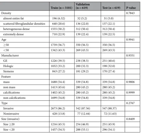
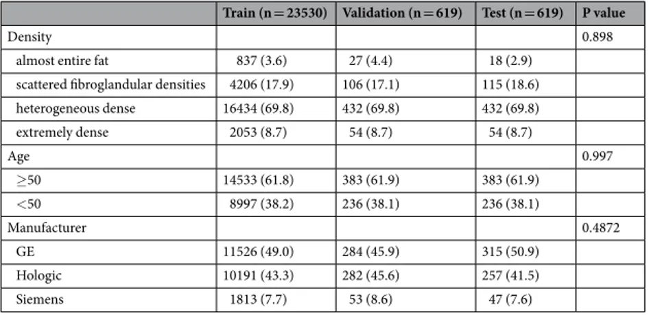
In 4,339 cancer cases, training, validation and test sets were randomly selected with a ratio of 5:1:1 (3,101/619/619). Each dataset was evenly distributed in terms of patients’ age, breast density, and manufac-turer, and cancer type, feature, and size in order to remove selection bias between training, validation and test sets (Table 1). Predominant features of cancer were mass (n = 2,366) or microcalcifications (n = 1,962), so other features (asymmetry for focal asymmetry (n = 463), distortion (n = 100)) were not controlled in the data sets.In 24,768 normal cases, the same number of validation (n = 619) and test (n = 619) cases were randomly selected, and the rest were used for training. For normal cases, each partition of the dataset was evenly distributed in terms of patients’ age, breast density, and manufacturer in order to remove selection bias (Table 2).
Development of the Algorithm.
Deep convolutional neural network (DCNN) is a deep learning algo-rithm specialized for images22. Each convolutional layer extracts features hierarchically (layer-by-layer) toabstract semantics from the raw input images. DIB-MG is implemented based on a residual network (ResNet)23,
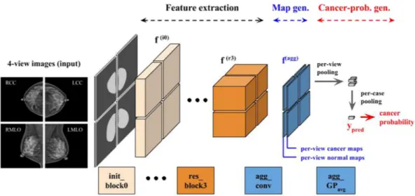
the state-of-the-art DCNN model for image recognition. Figure 1 shows the overall architecture of DIB-MG. It Train (n = 3101) Validation (n = 619) Test (n = 619) P value
Density 0.7843
almost entire fat 196 (6.32) 32 (5.2) 31 (5.0)
scattered fibroglandular densities 640 (20.6) 136 (22.0) 137 (22.1)
heterogeneous dense 1555 (50.2) 312 (50.4) 312 (50.4) extremely dense 710 (22.9) 139 (22.4) 139 (22.5) Age 0.9941 ≥50 1759 (56.7) 350 (56.5) 350 (56.5) <50 1342 (43.3) 269 (43.5) 269 (43.5) Manufacturer 0.9351 GE 1226 (39.5) 238 (38.5) 251 (40.6) Hologic 1032 (33.2) 200 (32.3) 198 (32.0) Siemens 843 (27.2) 181 (29.2) 170 (27.4) Feature mass 1688 (54.4) 339 (54.8) 339 (54.8) 0.9806 non mass 1413 (45.6) 280 (45.2) 280 (45.2) calcifications 1402 (45.2) 280 (45.2) 280 (45.2) 0.9999 non calcifications 1699 (54.8) 339 (54.8) 339 (54.8) Type 0.2767 Invasive 2673 (86.2) 542 (87.56) 547 (88.37) Noninvasive 428 (13.8) 77 (12.44) 72 (11.63) Size (invasive) 0.8409 Size ≥20 1216 (45.5) 254 (46.9) 251 (45.9) Size <20 1457 (54.5) 288 (53.1) 296 (54.1)
consists of two initial blocks (init_block), four residual blocks (residual_block), and an aggregation block (aggre-gate_block). Each residual block includes four consecutive convolution layers with skip connection as described in the right-bottom of the Fig. 1 (⊕ is an element-wise addition operator), while the other blocks include a single convolution layer. Each block also includes some auxiliary components such as a batch normalization layer (BN: normalization of activations within a batch)24, a rectified linear unit (ReLU: a simple mathematical function for
non-linear activation)22, a max-pooling layer (P
max: static dimension reduction function for translation-invariant feature abstraction)22, and a global-average-pooling (GP
avg: average of the entire 2-dimensional input feature map)23. Details of the components are well described in the original literatures22–24.
DIB-MG consists of nineteen convolution layers with a two-stage global-average-pooling layer. The former eighteen convolution layers extract hierarchical features for cancer classification, while the last convolution layer (1 × 1 convolution kernel with filter width 2) generates per-view maps (one for cancer, and the other for nor-mal cases) via for final DIB construction (Fig. 2). Figure 3 shows an example of DIB as well as ground-truth lesions. Since we did not use pixel-level lesion annotation in this experiment, each per-view map generated from the last convolution layer (i.e. map generation stage) was converted in a single value to be compared with the ground-truth label (biopsy-proven cancer: 1 or normal: 0). So, the final maps were converted into a vector (each vector element represents its own class) using the global-average-pooling operation. In the training stage, the error between the output vector (y_pred in Fig. 2) and the ground-truth label was propagated backward via back-propagation algorithm25, and the model parameters of the entire network were updated based on the
prop-agated errors.
Training Set-up.
All the DICOM files are first converted to PNG files considering window_center and win-dow_width defined in the header of each DICOM, and then the pixel values are normalized to be in the range −1.0 to 1.0. Random perturbation of the pixel intensity in terms of constrast (±10%) and brightness (±10%) is used every training iteration to overcome the difference in vendor-specific contrast/brightness characteristics. AllTrain (n = 23530) Validation (n = 619) Test (n = 619) P value
Density 0.898
almost entire fat 837 (3.6) 27 (4.4) 18 (2.9)
scattered fibroglandular densities 4206 (17.9) 106 (17.1) 115 (18.6)
heterogeneous dense 16434 (69.8) 432 (69.8) 432 (69.8) extremely dense 2053 (8.7) 54 (8.7) 54 (8.7) Age 0.997 ≥50 14533 (61.8) 383 (61.9) 383 (61.9) <50 8997 (38.2) 236 (38.1) 236 (38.1) Manufacturer 0.4872 GE 11526 (49.0) 284 (45.9) 315 (50.9) Hologic 10191 (43.3) 282 (45.6) 257 (41.5) Siemens 1813 (7.7) 53 (8.6) 47 (7.6)
Table 2. Demographics in normal cases.
the input images are downscaled to 1600 × 1600, i.e. rescaled to 1600 in terms of the longer side and zero-padded to be 1600 × 1600 (zero-padded on the left side of RCC/RMLO and the right side of LCC/LMLO).
Initial learning rate 0.001 is decayed by a factor of 5 every 10 epochs until the 30 epochs. Stochastic gradient descent (SGD) with momentum 0.9 is used for optimization. Minibatch size is 64 images (16 exams) based on eight graphic processing units (GPUs). Weight decay constant 0.0005 is used for regularization. All the experi-ment is done with TensorFlow26.
Evaluation of the Algorithm.
Training proceeds to minimize the prediction error of the entire training set, and the final DIB-MG performed best on the validation set is chosen for evaluation on the test set. In an inference stage, the final output value of the trained model (y_pred ranging from 0.0 to 1.0) is used to decide whether the input case is cancer or not. More specifically, y_pred represents the confidence level of malignancy. This value is not exactly equal to the probability of cancer, as cancer cannot be specified as a probability. But it is correlated with the cancer probability in real exams. The constructed DIB (class number of per-view maps generated from the last convolution layer) includes information on spatial discriminativity. As mentioned before, each map rep-resents the corresponding class and shows the most discriminative part in terms of the final classification result; e.g., if y_pred is 0.9 (cancer probability), then the region with the highest value on the cancer map is the most discriminative part in terms of its cancer decision.Figure 2. Hierarchical feature abstraction, DIB map generation, and cancer probability generation.
Figure 3. DIB example with ground-truth lesion. A 44-year-old woman with invasive ductal carcinoma of the right breast. A 22 mm-sized mass was correctly highlighted by DIB. The confidence score for cancer of DIB was 1.0 and 0.026 for the right and left breast.
Statistical Analysis and Performance Comparison.
Chi-square tests were used to see whether there was any difference in categorical variables between training, validation and test sets. With validation and test sets, diagnostic performances were measured. Sensitivity, specificity, and accuracy were compared according to vari-ous demographics using the chi-square test. For features, logistic regression with the generalized estimating equa-tion (GEE) method was applied to take into account that some patients had mass with microcalcificaequa-tions. The AUC were compared between the validation and test sets using chi-square statistics. All analyses were conducted by a statistician using SAS statistical software (version 9.4; SAS Institute Inc., Cary, NC, USA) and R version 3.3.1 (R Foundation for Statistical Computing, Vienna, Austria).Results
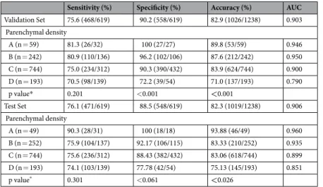
At the operating point (threshold) of 0.5, sensitivity was 75.6% and 76.1% when specificity was 90.2% and 88.5%, and AUC was 0.903 and 0.906 for the validation and test sets, respectively, with no statistical difference (Table 3). Sensitivity and specificity were not statistically significant between age ≥50 and <50, but they were significantly different according to the manufacturer (Table 3). In regards to breast density, sensitivity was not affected, how-ever, specificity and accuracy decreased as breast density increased (Table 4).
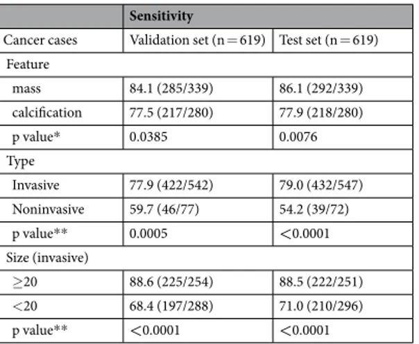
In the malignant group (Table 5), sensitivity was better in mass than in calcifications (84.1–86.1% vs 77.5– 77.9%), better in invasive cancer than in non-invasive cancer (77.0–77.9% vs 54.2–59.7%), and better in mass ≥20 mm than <20 mm (88.5–88.6%, 68.4–71.0%).
Sensitivity (%) Specificity (%) Accuracy (%) AUC
Validation Set 75.6 (468/619) 90.2 (558/619) 82.9 (1026/1238) 0.903 Age ≥50 77.1 (270/350) 91.9 (352/383) 84.9 (622/733) 0.914 <50 73.6 (198/269) 87.3 (206/236) 80.0 (404/505) 0.882 p value* 0.310 0.061 0.026 0.080 Manufacturer GE 77.5 (186/240) 91.1 (257/282) 84.9 (443/522) 0.924 Hologic 63.6 (126/198) 93.3 (265/284) 81.1 (391/482) 0.863 Siemens 86.2 (156/181) 67.9 (36/53) 82.1 (192/234) 0.861 p value* <0.0001 <0.0001 0.2704 Test Set 76.1 (471/619) 88.5 (548/619) 82.3 (1019/1238) 0.906 Age ≥50 76.3 (267/350) 90.1 (345/383) 83.5 (612/733) 0.911 <50 75.83 (204/269) 86.01 (203/236) 80.6 (407/505) 0.897 p value* 0.897 0.124 0.189 0.395 Manufacturer GE 74.6 (188/252) 89.1 (229/257) 81.9 (417/509) 0.910 Hologic 67.0 (132/197) 92.1 (290/315) 82.4 (422/512) 0.880 Siemens 88.8 (151/170) 61.7 (29/47) 83.0 (180/217) 0.888 p value* <0.0001 <0.0001 0.943
Table 3. Diagnostic Performances according to age and manufacturer. *chi-square test. Sensitivity (%) Specificity (%) Accuracy (%) AUC
Validation Set 75.6 (468/619) 90.2 (558/619) 82.9 (1026/1238) 0.903 Parenchymal density A (n = 59) 81.3 (26/32) 100 (27/27) 89.8 (53/59) 0.946 B (n = 242) 80.9 (110/136) 96.2 (102/106) 87.6 (212/242) 0.950 C (n = 744) 75.0 (234/312) 90.3 (390/432) 83.9 (624/744) 0.900 D (n = 193) 70.5 (98/139) 72.2 (39/54) 71.0 (137/193) 0.790 p value* 0.201 <0.001 <0.001 Test Set 76.1 (471/619) 88.5 (548/619) 82.3 (1019/1238) 0.906 Parenchymal density A (n = 49) 90.3 (28/31) 100 (18/18) 93.88 (46/49) 0.960 B (n = 252) 75.9 (104/137) 92.17 (106/115) 83.33 (210/252) 0.935 C (n = 744) 75.6 (236/312) 88.43 (382/432) 83.06 (618/744) 0.899 D (n = 193) 74.1 (103/139) 77.78 (42/54) 75.13 (145/193) 0.851 p value* 0.301 <0.061 <0.026
Discussions
This is the first study that applies deep learning algorithms in mammography without pixel-level supervision. Our results showed that the AUC values for diagnosing breast cancer using the DIB-MG algorithm were 0.903–0.906, which demonstrates that DIB-MG algorithms can be trained with large-scale data sets without pre-defined mam-mographic features.
Deep learning algorithm in mammography have been previously studied by several researchers. Wang et al. reported that breast cancers presenting microcalcifications could be discriminated by deep learning27. They used
a previously reported computerized segmentation algorithm in order to extract the clustered microcalcifications from mammograms28. In their approach, pre-defined microcalcification features obtained from lesion-annotated
mammograms were used as an input for the unsupervised deep learning model (stacked autoencoder)29. Kooi
et al. compared state-of-the art mammography CAD systems, relying on manually designed features as well as data-driven features using DCNN18. Especially in a deep learning approach, image patches extracted from
lesion-annotated mammograms were used for training. Becker et al. evaluated the diagnostic performance of their deep neural network model for breast cancer detection30. A total 143 histology-proven cancers and 1,003
normal cases were used for this study, where all the cancer cases of the training dataset were manually annotated pixel-wise by radiologists according to descriptions in the radiology report. Compared to the aforementioned approaches, we used pure data-driven features from raw mammograms without any lesion annotations, which is scalable and practical for future CAD systems.
In previous reports with CAD, sensitivity was higher in microcalcifications than mass31–34, however, in this
study, sensitivity was better in mass than calcifications. That is due to the difference in data sets. In our data set, both screening and diagnostic mammograms were included, in which 45.7% (1721/3762) of invasive carcinomas were equal or larger than 2 cm, whereas other studies with CAD included only screening mammograms31–34.
Further studies using the DIB-MG algorithm on screening data sets should follow.
Our data showed that sensitivity for breast cancer detection was similar for non-dense breasts and dense breasts. However, specificity decreased as breast density increased. Eventually, low specificity was directly related with increasing false-positives, so we need to develop algorithms increasing specificity in the future.
In our study, diagnostic performance was different according to the manufacturer; sensitivity is the highest (88.8%) and specificity is the lowest (61.7%) in Siemens. In each data set (training, validation and test sets), the three manufacturers were evenly distributed (roughly 4:3:3 in cancer cases, 5:4:1 in normal cases). However, can-cer cases were occupied with 27.2–29.2%, compared to 7.6–8.6% in normal cases in Siemens machine. This indi-cates that the number of cases trained with a certain type of machine can influence the diagnostic performance of mammography. This kind of selection bias should be considered in a future study regarding deep learning.
We acknowledge several limitations of our study. First, in this study we included only normal and cancer cases, so benign cases need to be included. Also, the dataset should be more expanded. Second, our model does not use any pixel-level annotations for training, so there might be errors in predicting the lesion location in examples predicted as cancer. It is necessary to confirm whether the lesion location is accurately predicted, and retrain the model based on those examples to improve localization performance.
In conclusion, this research showed the potential of DIB-MG as a screening tool for breast cancer. Further studies using a large number of high-quality data including benign cases are needed to further investigate its feasibility as a screening tool.
References
1. Hendrick, R. E., Smith, R. A., Rutledge, J. H., III & Smart, C. R. Benefit of screening mammography in women aged 40–49: a new meta-analysis of randomized controlled trials. Journal of the National Cancer Institute. Monographs 87–92 (1997).
2. Tabar, L. et al. Beyond randomized controlled trials: organized mammographic screening substantially reduces breast carcinoma mortality. Cancer 91, 1724–1731 (2001).
3. Oeffinger, K. C. et al. Breast Cancer Screening for Women at Average Risk: 2015 Guideline Update From the American Cancer Society. Jama 314, 1599–1614, https://doi.org/10.1001/jama.2015.12783 (2015).
Sensitivity
Cancer cases Validation set (n = 619) Test set (n = 619) Feature mass 84.1 (285/339) 86.1 (292/339) calcification 77.5 (217/280) 77.9 (218/280) p value* 0.0385 0.0076 Type Invasive 77.9 (422/542) 79.0 (432/547) Noninvasive 59.7 (46/77) 54.2 (39/72) p value** 0.0005 <0.0001 Size (invasive) ≥20 88.6 (225/254) 88.5 (222/251) <20 68.4 (197/288) 71.0 (210/296) p value** <0.0001 <0.0001
Table 5. Diagnostic Performances according to malignant characteristics. *Logistic regression using GEE, **chi-square test.
4. Nelson, H. D. et al. Effectiveness of Breast Cancer Screening: Systematic Review and Meta-analysis to Update the 2009 U.S. Preventive Services Task Force Recommendation. Annals of internal medicine 164, 244–255, https://doi.org/10.7326/M15-0969
(2016).
5. Siu, A. L. & Force, U. S. P. S. T. Screening for Breast Cancer: U.S. Preventive Services Task Force Recommendation Statement. Annals
of internal medicine 164, 279–296, https://doi.org/10.7326/M15-2886 (2016).
6. D’Orsi, C. J., Sickles, E. A., Mendelson, E. B., Morris, E. A. ACR BI-RADS atlas, breast imaging reporting and data system, 5th. (Reston, VA: American College of Radiology, 2013).
7. Beam, C. & Sullivan, D. Variability in mammogram interpretation. Adm Radiol J 15, 47, 49–50, 52 (1996).
8. Breast Cancer Surveillance Consortium. Smoothed plots of sensitivity (among radiologists finding 30 or more cancers), 2004–2008—based on BCSC data through 2009. National Cancer Institute; website. breastscreening.cancer.gov/data/benchmarks/ screening/2009/figure 10.html. Last modified July 9, 2014.
9. Leung, J. W. et al. Performance parameters for screening and diagnostic mammography in a community practice: are there differences between specialists and general radiologists? AJR Am J Roentgenol 188, 236–241, https://doi.org/10.2214/AJR.05.1581
(2007).
10. Freer, T. W. & Ulissey, M. J. Screening mammography with computer-aided detection: prospective study of 12,860 patients in a community breast center. Radiology 220, 781–786, https://doi.org/10.1148/radiol.2203001282 (2001).
11. Petrick, N. et al. Breast cancer detection: evaluation of a mass-detection algorithm for computer-aided diagnosis–experience in 263 patients. Radiology 224, 217–224, https://doi.org/10.1148/radiol.2241011062 (2002).
12. Birdwell, R. L., Bandodkar, P. & Ikeda, D. M. Computer-aided detection with screening mammography in a university hospital setting. Radiology 236, 451–457, https://doi.org/10.1148/radiol.2362040864 (2005).
13. Morton, M. J., Whaley, D. H., Brandt, K. R. & Amrami, K. K. Screening mammograms: interpretation with computer-aided detection–prospective evaluation. Radiology 239, 375–383, https://doi.org/10.1148/radiol.2392042121 (2006).
14. Fenton, J. J. et al. Short-term outcomes of screening mammography using computer-aided detection: a population-based study of medicare enrollees. Annals of internal medicine 158, 580–587, https://doi.org/10.7326/0003-4819-158-8-201304160-00002 (2013). 15. Rao, V. M. et al. How widely is computer-aided detection used in screening and diagnostic mammography? J Am Coll Radiol 7,
802–805, https://doi.org/10.1016/j.jacr.2010.05.019 (2010).
16. Cole, E. B. et al. Impact of computer-aided detection systems on radiologist accuracy with digital mammography. AJR Am J
Roentgenol 203, 909–916, https://doi.org/10.2214/AJR.12.10187 (2014).
17. Lehman, C. D. et al. Diagnostic Accuracy of Digital Screening Mammography With and Without Computer-Aided Detection.
JAMA Intern Med 175, 1828–1837, https://doi.org/10.1001/jamainternmed.2015.5231 (2015).
18. Kooi, T. et al. Large scale deep learning for computer aided detection of mammographic lesions. Med Image Anal 35, 303–312,
https://doi.org/10.1016/j.media.2016.07.007 (2017).
19. Bengio, Y., Courville, A. & Vincent, P. Representation learning: a review and new perspectives. IEEE Trans Pattern Anal Mach Intell
35, 1798–1828, https://doi.org/10.1109/TPAMI.2013.50 (2013).
20. LeCun, Y., Bengio, Y. & Hinton, G. Deep learning. Nature 521, 436–444, https://doi.org/10.1038/nature14539 (2015).
21. Schmidhuber, J. Deep learning in neural networks: an overview. Neural Netw 61, 85–117, https://doi.org/10.1016/j.neunet. 2014.09.003 (2015).
22. Krizhevsky A, S. I. & Hinton, G. E. ImageNet Classification with Deep ConvolutionalNeural Networks. Neural Information
Processing Systems (NIPS) (2012).
23. He, K., Zhang, X., Ren, S. & Sun, J. Deep residual learning for image recognition. In Conference on Computer Vision and Pattern
Recognition (CVPR) (2016).
24. Ioffe, S. & Szegedy, C. Batch normalization: Accelerating deep network training by reducing internal covariate shift. In International
Conference on Machine Learning (ICML) (2015).
25. Hornik, K., Halbert, S. M. & Multilayer, W. feedforward networks are universal approximators. Neural networks Neural networks 2, 359–366 (1989).
26. Abadi, M. et al. TensorFlow: Large-scale machine learning on heterogeneous systems. Software available from tensorflow.org (2015). 27. Wang, J. et al. Discrimination of Breast Cancer with Microcalcifications on Mammography by Deep Learning. Sci Rep 6, 27327,
https://doi.org/10.1038/srep27327 (2016).
28. Shao, Y. Z. et al. Characterizing the clustered microcalcifications on mammograms to predict the pathological classification and grading: a mathematical modeling approach. J Digit Imaging 24, 764–771, https://doi.org/10.1007/s10278-011-9381-2 (2011). 29. Vincent, P., Larochelle, H., Lajoie, I., Bengio, Y. & Manzagol, P. A. Stacked Denoising Autoencoders: Learning Useful Representations
in a Deep Network with a Local Denoising Criterion. J Mach Learn Res 11, 3371–3408 (2010).
30. Becker, A. S. et al. Deep Learning in Mammography: Diagnostic Accuracy of a Multipurpose Image Analysis Software in the Detection of Breast Cancer. Investigative radiology https://doi.org/10.1097/rli.0000000000000358 (2017).
31. Sadaf, A., Crystal, P., Scaranelo, A. & Helbich, T. Performance of computer-aided detection applied to full-field digital mammography in detection of breast cancers. Eur J Radiol 77, 457–461, https://doi.org/10.1016/j.ejrad.2009.08.024 (2011). 32. Kim, S. J. et al. Computer-aided detection in digital mammography: comparison of craniocaudal, mediolateral oblique, and
mediolateral views. Radiology 241, 695–701, https://doi.org/10.1148/radiol.2413051145 (2006).
33. Murakami, R. et al. Detection of breast cancer with a computer-aided detection applied to full-field digital mammography. J Digit
Imaging 26, 768–773, https://doi.org/10.1007/s10278-012-9564-5 (2013).
34. Yang, S. K. et al. Screening mammography-detected cancers: sensitivity of a computer-aided detection system applied to full-field digital mammograms. Radiology 244, 104–111, https://doi.org/10.1148/radiol.2441060756 (2007).
Acknowledgements
This work was partly supported by Institute for Information & Communications Technology Promotion(IITP) grant funded by the Korea government(MSIP) (Title: Diagnosis Support System with Hospital-Scale Medical Data and Deep Learning), and partly supported by the research project funded by Lunit Inc. (Title: Study of Verification and Validation of Deep Learning Based Breast Image Diagnosis Support Algorithm).
Author Contributions
All authors were responsible for the study concept. E.-K.K. and H.-E.K. contributed to the study design. E.-K.K. B.J.K., Y.-M.S., O.H.W., C.W.L. contributed to the data collection and wrote the first draft of the manuscript. H.-E.K., E.-K.K. and K.H. contributed to the statistical analysis. All authors reviewed and approved the final draft of the manuscript.
Additional Information
Publisher's note: Springer Nature remains neutral with regard to jurisdictional claims in published maps and institutional affiliations.
Open Access This article is licensed under a Creative Commons Attribution 4.0 International License, which permits use, sharing, adaptation, distribution and reproduction in any medium or format, as long as you give appropriate credit to the original author(s) and the source, provide a link to the Cre-ative Commons license, and indicate if changes were made. The images or other third party material in this article are included in the article’s Creative Commons license, unless indicated otherwise in a credit line to the material. If material is not included in the article’s Creative Commons license and your intended use is not per-mitted by statutory regulation or exceeds the perper-mitted use, you will need to obtain permission directly from the copyright holder. To view a copy of this license, visit http://creativecommons.org/licenses/by/4.0/.