Retrospective evaluation of whole exome and genome mutation calls in 746 cancer samples

Retrospective evaluation of whole exome and

genome mutation calls in 746 cancer samples

Matthew H. Bailey

1,2,3

, William U. Meyerson

4,5

, Lewis Jonathan Dursi

6,7

, Liang-Bo Wang

1,2

,

Guanlan Dong

2

, Wen-Wei Liang

1,2

, Amila Weerasinghe

1,2

, Shantao Li

5

, Yize Li

1

, Sean Kelso

2

,

MC3 Working Group*, PCAWG novel somatic mutation calling methods working group*, Gordon Saksena

8

,

Kyle Ellrott

9

, Michael C. Wendl

1,10,11

, David A. Wheeler

12,13

, Gad Getz

8,14,15,16

, Jared T. Simpson

6,17

,

Mark B. Gerstein

5,18,19

✉

, Li Ding

1,2,3,20

✉

& PCAWG Consortium*

The Cancer Genome Atlas (TCGA) and International Cancer Genome Consortium (ICGC)

curated consensus somatic mutation calls using whole exome sequencing (WES) and whole

genome sequencing (WGS), respectively. Here, as part of the ICGC/TCGA Pan-Cancer

Analysis of Whole Genomes (PCAWG) Consortium, which aggregated whole genome

sequencing data from 2,658 cancers across 38 tumour types, we compare WES and WGS

side-by-side from 746 TCGA samples,

finding that ~80% of mutations overlap in covered

exonic regions. We estimate that low variant allele fraction (VAF < 15%) and clonal

het-erogeneity contribute up to 68% of private WGS mutations and 71% of private WES

mutations. We observe that ~30% of private WGS mutations trace to mutations identi

fied by

a single variant caller in WES consensus efforts. WGS captures both ~50% more variation in

exonic regions and un-observed mutations in loci with variable GC-content. Together, our

analysis highlights technological divergences between two reproducible somatic variant

detection efforts.

https://doi.org/10.1038/s41467-020-18151-y

OPEN

1_{The McDonnell Genome Institute at Washington University, St. Louis, MO 63108, USA.}2_{Division of Oncology, Department of Medicine, Washington}

University School of Medicine, St. Louis, MO 63108, USA.3Alvin J. Siteman Cancer Center, Washington University School of Medicine, St. Louis, MO 63108,

USA.4Yale School of Medicine, Yale University, New Haven, CT 06520, USA.5Program in Computational Biology and Bioinformatics, Yale University, New

Haven, CT 06520, USA.6Computational Biology Program, Ontario Institute for Cancer Research, Toronto, ON M5G 0A3, Canada.7The Hospital for Sick

Children, Toronto, ON M5G 1X8, Canada.8Broad Institute of MIT and Harvard, Cambridge, MA 02142, USA.9Biomedical Engineering, Oregon Health and

Science University, Portland, OR 97239, USA.10Department of Mathematics, Washington University in St. Louis, St. Louis, MO 63130, USA.11Department of

Genetics, Washington University School of Medicine, St.Louis, MO 63110, USA.12Human Genome Sequencing Center, Baylor College of Medicine, Houston,

TX 77030, USA.13Department of Molecular and Human Genetics, Baylor College of Medicine, Houston, TX 77030, USA.14Harvard Medical School, Boston,

MA 02115, USA.15Center for Cancer Research, Massachusetts General Hospital, Boston, MA 02114, USA.16Department of Pathology, Massachusetts

General Hospital, Boston, MA 02114, USA.17_{Department of Computer Science, University of Toronto, Toronto, ON M5S, Canada.}18_{Department of}

Computer Science, Yale University, New Haven, CT 06520, USA.19_{Department of Molecular Biophysics and Biochemistry, Yale University, New Haven, CT}

06520, USA.20_{Department of Medicine and Department of Genetics, Washington University School of Medicine, St. Louis, MO 63110, USA. *Lists of}

authors and their affiliations appear at the end of the paper. ✉email:mark.gerstein@yale.edu;lding@wustl.edu

123456789

C

omplementary efforts of The Cancer Genome Atlas

(TCGA) and the International Cancer Genome

Con-sortium (ICGC) have recently produced two of the highest

quality and most elaborate and reproducible somatic variant call

sets from exome and whole genome-level data in cancer

geno-mics, respectively. The motivation for these efforts stems from the

notion that

“scientific crowd sourcing” and combining mutation

callers can provide very strong results.

These two efforts produced variant calls from 10 different

callers, namely Radia

1

_{, Varscan}

2

_{, MuSE}

3

_{, MuTect}

4

_{, Pindel}

5,6

_,

Indelocator

7

, SomaticSniper

8

for WES and MuSE,

Broad-Pipeline (anchored by MuTect), Sanger-pipeline, German

Cancer Research Center pipeline (DKFZ), and SMuFin

9

_{, for}

WGS. Briefly, the PCAWG Consortium aggregated whole

genome sequencing data from 2658 cancers across 38 tumor

types generated by the ICGC and TCGA projects. These

sequencing data were re-analyzed with standardized,

high-accuracy pipelines to align to the human genome (reference

build hs37d5) and identify germline variants and somatically

acquired mutations

10

_{. Of the 885 TCGA samples in ICGC, 746}

were included in the latest exome call set produced by both the

Multi-Center Mutation Calling in Multiple Cancers (MC3)

effort and the Pan-Cancer Analysis of Whole Genomes

(PCAWG) Consortium set. These 746 samples represent a

critical benchmark for high-level analysis of similarities and

differences between exome and genome somatic variant

detection methods.

Reproducibility of mutations identified by both whole exome

capture sequencing and whole genome sequencing (WGS)

techniques remains an important issue, not only for the

scien-tific use of large, established data sets, but for data designs of

future research projects. Previous work analyzing exome capture

effects on sequence read quality has shown that GC-content bias

is the major source of variation in coverage

11

. A performance

comparison across exome-captured platforms demonstrated

that for most technologies, both high and low GC-content result

in reduced coverage in read depth

12

. Belkadi et al. compared

mutation calls between WGS and WES, observing that ~3% of

coding variants with high quality were only detected in WGS,

and WGS also had a more uniform distribution of coverage

depth, genotype quality, and minor read ratio

13

_{. Furthermore,}

due to the relatively high error rate per read in next-generation

sequencing

14

_{, the detectability of mutations with low variant}

allele fractions (VAFs) is limited by background noise. Despite

these studies’ nuanced preference towards WGS, others contend

that WES will remain a better choice until costs of WGS fall

15

_.

The decision to sequence exomes or whole genomes is further

confounded as more recent publications in oncology select

either WGS

16–20

_{or WES}

21–24

_{. Recognizing the unresolved}

nature of this issue, Schwarze et al. have called for more

com-prehensive studies comparing the WES and WGS studies,

especially as this issue has important ramifications for the

clinic

25

.

Our analysis provides confidence that mutation calls within

the captured exonic regions of these two data sets are

largely consistent. We highlight common sample, cohort, and

caller-specific challenges in cancer variant detection from the

TCGA and ICGC efforts. We show that variants that are

most confidently called in one database i.e., called by multiple

callers, are very likely to be called in the other. We assess

how reproducibility impacts higher-level mutation signature

analysis and illustrate the need for caution in assessing

perfor-mance that can only be identified by the overlap of these two

data sets. Finally, we explore the capacity of WGS to detect

recurrent non-coding mutations captured by whole exome

sequencing.

Results

Data and workflow. We used publicly available data from the

MC3 and PCAWG repositories, consisting of ~3.6 M and ~47 M

variants, respectively (Fig.

1

a). 746 samples were sequenced by

both WES and WGS, comprising various aliquots and portions of

the same tumor (Supplementary Data 1, Fig.

1

b). Effects of these

differences are discussed below for preliminary results, but we

ultimately used the entire set of 746 samples in the variant

overlap analysis, since the effects of tumor partitioning did not

play a significant role (Supplementary Fig. 1). By restricting the

public data sets to overlapping samples, we reduced the total

corpus to ~220 K (6.1%) and ~23 M (49.6%) mutations for exome

and whole genome, respectively. It is notable that there is an

enrichment of variants in hypermutated samples from COAD,

HNSC, LUAD, and STAD in the PCAWG set used in this study

(Supplementary Fig. 2). To begin building a comparable set of

mutations between these two studies, we further restricted the

whole genome data set to exon regions provided by the MC3

analysis working group. This reduced the WGS data set to 1.6% of

its original size, within range of total exome material

estima-tions

26

(Fig.

1

a). The next step involved removing poorly-covered

variants potentially caused by technical anomalies by limiting

mutations to those captured in coverage

files (distributed as.wig

files). A reciprocal coverage strategy was used, meaning PCAWG

mutations were restricted to covered genomic regions in MC3

and vice versa, thereby maintaining a complementary set of

callable genomic regions. Removal of mutations in uncovered

regions reduced the remaining PCAWG data set by

approxi-mately one-half, from 387,166 to 183,424 mutations. We also

identified 4241 MC3 and 2219 PCAWG mutations that were

present in the respective MAF but were not marked as covered in

the coverage

files provided by a single group. This suggests that

different tools consider different minimum coverage strategies.

These mutations reflect 2.0% and 1.2%, respectively, of the total

mutation discrepancy and were removed because some callers

had limited capacity to identify mutations in poorly-covered

regions (see

“Methods” section). Finally, filter flags provided by

MC3 were used to assess somatic mutation

filtering strategies. At

this stage, we performed

filter optimization to comprehensively

evaluate all possible combinations of MC3

filters (Supplementary

Fig. 3a). Ultimately, we decided to only remove OxoG labeled

artifacts and duplicated events produced by these

filters (see

“Methods” section, Supplementary Data 2). Since each stage of

this

filtering workflow resulted in many alternative decisions and

outcomes, we built MAFit, a web-based graphical user interface

that allows users to easily customize comparisons of merged

mutations (

https://mbailey.shinyapps.io/MAFit/

). A MC3

filter

assessment also shows that many variants with

filter flags in MC3

are present in the PCAWG variant call set, suggesting a need for

improved

filtering strategies (Supplementary Fig. 3b).

TCGA samples comprise a sizable fraction of the PCAWG

sample pool (~30%, Supplementary Data 1) Additional WGS

sequencing from TCGA allowed for mutation validation

27

and

insights into non-coding mutations, such as in TET2. However,

this selection process could have potentially influenced our basic

comparison of exome-sequenced samples and genome-sequenced

samples in two fundamental ways. First, vagaries of tumor

extraction and tissue storage protocols may have resulted in many

different portions of a tumor being stored, introducing the

possibility that different subclones of the same tumor could be

present. These could have very different genetic makeups. This

information was captured in different substrings of the TCGA

identification barcode (see “Methods” section). From the 746

TCGA barcodes, we found that 64% (477) could be traced to the

same well of a microtiter plate (Fig.

1

b). After correcting for

cancer type, we modeled both the impact of matching barcode

identifiers between MC3 and PCAWG and variant concordance,

finding that differing barcodes did not have an appreciable

impact. This result was seen for all samples, even when excluding

the hypermutator (Fig.

1

). Second, each AWG was able to

independently select samples for WGS, which, while not affecting

mutation calling, does raise potential biases when comparing

PCAWG results to TCGA exome cohort data. An enrichment

analysis was performed to identify which tumor subtypes may

have been preferentially selected for different cancer types. We

found that four tumor subtypes were enriched in the PCAWG

effort from TCGA samples: infiltrating ductal breast cancer,

endometrial serous adenocarcinoma, differentiated liposarcoma,

and

low

grade

oligodendroglioma

(FDR < 0.05,

Fig.

1

c,

Supplementary Data 3, and see

“Methods” section). Final tumor

sample counts for each cancer type are shown in Fig.

1

d.

Landscape of mutational overlap between WGS and WES calls.

Limiting our analysis to coding regions with sufficient coverage

yielded a total of 202,459 variants (155,859 matched, 21,627

unique MC3 variants, and 24,973 unique PCAWG mutations),

with 76.7% in concordance between MC3 and PCAWG and

10.7% and 12.3% being unique in MC3 and PCAWG, respectively

(Fig.

2

a). Concordance can be further separated into SNPs and

indels, with 79% and 57% overlapping, respectively

(Supple-mentary Fig. 4). Variant overlap was further investigated to reveal

Tissue Vial Portion AnalytePlate

500 550 600 650 700 750

Matched sample count

0

TCGA Barcode =TCGA–DD–0001–01B–01D–A152

MC3 Variants PCAWG Variants

46,607,230 23,137,829 387,166 183,424 181,976 180,832 3,600,964 219,567 219,567 214,675 210,435 177,486 Overlapping samples Reduce to exons MC3 MAF MC3 MAF Merged MAF PCAWG MAF 155,859 Unique 21,627 Unique 24,973 PCAWG MAF

BRCA: Infiltrating Lobular _{BRCA: Infiltrating Ductal}

LGG: Astrocytoma

LGG: Oligodendroglioma

LGG: Oligoastrocytoma

SARC: Dedifferentiated liposarcoma

STAD: Papillary Type

THCA: Classical/usual THCA: Follicular

UCEC: Endometrioid adenocarcinoma

UCEC: Serous adenocarcinoma

0 2 4 6 −2 0 2 log2(Odds Ratio) −log10( P −value)

Higher represention than MC3

Lower represention than MC3

0 22 86 20 0 33 6 0 33 42 43 2732 18 51 36 47 0 26 0 0 19 12 30 37 36 0 48 0 43 0 0 0 25 50 75 ACC

BLCA BRCA CESC CHOL COAD DLBC ESCA GBM HNSC KICH KIRC KIRP LGG LIHC LUAD LUSC _MESO

O

V

PAAD PCPG PRAD READ SARC SKCM STAD TGCT THCA THYM UCEC UCS UVM

TCGA cancer types

Number of samples Optimized filters & de-duplication Coverage reduction

a

b

c

d

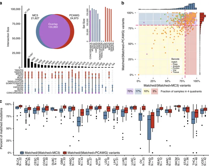
Fig. 1 Work_{flow and sample inclusion statistics. a A workflow diagram illustrates the number of mutations present during each step (gradient) of the}

filtering processes for MC3 (left, blue) and PCAWG (right, red). A brief description of each step of the intersection process is shown in between. b TCGA barcodes and aliquot IDs were used to match somatic sequencing. The exact match of these IDs is shown for various collection aliquots from tissue to

plate.c A volcano plot highlights cancer subtype discrepancy between each PCAWG and MC3 with−log10(p-value) on the y-axis and log2(odds ratio) on

the_{x-axis (Fisher’s exact test). The horizontal red bar indicates a significant threshold after multiple testing correction. Positive values indicate an}

over-representation of a cancer subtype in PCAWG, while negative values indicate an under-over-representation of a cancer subtype in PCAWG compared to

its association with mutation caller, sample, and cancer type

(Fig.

2

a–c). Consensus variant calling showed 91,705 (45.3%)

concordant variants were captured in the intersection of Sanger,

MuSE, DKFZ, and Broad callers from PCAWG, as well as

Varscan, SomaticSniper, Radia, MuTect, and MuSE callers from

MC3. Notably, an additional 7.7% were identified by all SNV

mutation detection algorithms, except SomaticSniper. The

reduced sensitivity of SomaticSniper is related to its algorithmic

consideration of tumor contamination in the matched normal

(e.g., skin) for liquid tumors

8

_{. After optimizing for}

_filtering

strategies, we performed a sample level comparison and found

that 70% of samples had greater than 80% mutation concordance

across the two cohorts. An additional 20% of samples had greater

than 80% mutation recoverability in one or the other technique

(Fig.

2

b). Skin Cutaneous Melanoma performed the best among

all cancer types and had the highest variant-matching rates for

both MC3 and PCAWG (Fig.

2

c). Generally, when considering all

MC3 and all PCAWG mutations separately, we observed that

PCAWG variant matching rates were generally higher, especially

for Kidney Chromophobe (KICH), Brain Lower Grade Glioma

(LGG), Ovarian Serous Cystadenocarcinoma (OV), Rectum

Adenocarcinoma (READ), and Thyroid Carcinoma (THCA). The

differences in OV are likely driven by whole genome amplified

library preparation. Generally, the median fractions for matching

MC3 variants were lower than those of matching PCAWG

var-iants. This result was unexpected because MC3 provided fewer

unique variants overall, suggesting that a large fraction of

PCAWG unique variants reside in a few samples. Furthermore,

after accounting for hypermutators, we identified a correlation

between non-silent mutations per megabase and mean consensus

percentages at the cancer level in both PCAWG consensus

per-centages (Mann–Whitney p-value = 1.97 × 10

−3

_{) and MC3}

con-sensus percentages (Mann–Whitney p-value = 6.59 × 10

−4

_{, see}

“Methods” section, Supplementary Fig. 1c, d). Despite strong

rank statistics, neither set exhibited strong correlation values for

MC3 variants or PCAWG variants, R

2

statistics

= 0.31 and 0.17

91,705 15,667 9855 72095658 475940563894348132493142300528672845221320542010197615721295115010291002909 885 875 784 0 25,000 50,000 75,000 100,000 Intersection Size CONCORDANCEMUTECT MUSE VARSCANRADIA SOMATICSNIPER*INDELOCATOR *PINDELMUSE DKFZ BROAD SANGER *SMUFIN CONCORDANCE MUTECT MUSE VARSCAN RADIA SOMATICSNIPER *INDELOCATOR *PINDEL MUSE DKFZ BROAD SANGER *SMUFIN 0 50,000 1 00,000 150,000 Set Size Overlap 155,860 PCAWG 24,973 MC3 21,627 0% 25% 50% 75% 100%

BLCA N = 22 BRCA N = 85 CESC N = 20 COAD N = 30 DLBC N = 6 GBM N = 33 HNSC N = 42 KICH N = 43 KIRC N = 27 KIRP N = 32 LGG N = 18 LIHC N = 51 LUAD N = 36 LUSC N = 47 OV N = 25 PRAD N = 19 READ N = 12 SARC N = 30 SKCM N = 37 STAD N = 36 THCA N = 48 UCEC N = 42

Percent of matched mutations

Matched/(Matched+MC3) Matched/(Matched+PCAWG) variants

0% 25% 50% 75% 100% 0% 25% 50% 75% 100% Matched/(Matched+MC3) variants Matched/(Matched+PCAWG) variants

Fraction of samples in 4 quadrants 70% 17% 10% 3% Barcode match Plate Analyte Portion Vial Tissue

a

b

c

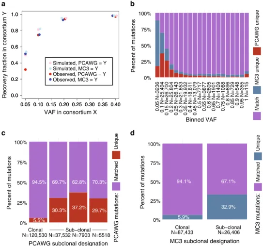
Fig. 2 Landscape of mutations overlap by caller, sample and cancer type. a UpSetR41_{plot shows the variant calling set intersection by caller. The y-axis}

indicates set intersection size and thex-axis uses a connected dot plot to indicate which sets are considered. Only the largest 27 intersecting sets are

shown. Two insets of the UpSetR plot highlight a classic Euler diagram (left), which indicates the total number of overlapping mutations. A set-size bar chart (right) illustrates the total number of mutations considered from each caller. The concordance set indicates the agreement between WES and WGS.

Indel callers are indicated with an asterisk.b A scatter plot shows the amount of concordance by sample by calculating the fraction of matched variants

divided by the total number of mutations made by MC3 exome sequencing and PCAWG whole genome sequencing (x and y-axis, respectively) below the

total fraction of samples within each quadrant. Each point within the plot is related to tumor portion data collected from the TCGA barcode ID.c As shown

above, this box plot separates panel b by cancer types (blue considers all MC3 variants, and red boxes indicate all PCAWG variants). Sample sizes are displayed for each cancer; points indicate samples that extend past 1.5 times the interquartile range; and horizontal bars within each box and whisker indicates median matched mutation fraction.

respectively with the majority of cancer types exceeding 80%

mean concordance. Thus, one may expect to observe slightly

higher variant

fidelity in samples with more mutations.

Variant allele fraction affects call-rates. After achieving a

comparable data set and merging MC3 and PCAWG variants, we

found that low VAF is the prevailing attribute of unique

muta-tions. VAF is a fundamental factor in somatic variant detection,

as well as sub-clonal structure prediction, and is used to predict

subclonal tumor growth rates and metastatic potential. To explore

the contribution of VAF, we sought to distinguish the

contribu-tion of subclonal structure and statistical chance when exploring

private mutations in a single call set. We articulate our

findings in

six broad categories: modeling sequence noise, departure from

idealized behavior, sub-clonal modeling, annotation differences,

variant-caller effects, and analysis correlations.

Association of variant allele fraction with recoverability. We

have observed that variants with low VAF are less likely to be

reported in both call-sets. This

finding relates to the lower

sen-sitivity of somatic variant callers for variants with low VAF. To

illustrate this principle, we estimated the expected overlap rate

between MC3 and PCAWG at different VAFs. The sensitivity of

MuSE across a range of VAFs and read depths in synthetic data

was reported in Fan et al., 2016

3

_{. We used these reported}

benchmarking characteristics of MuSE to estimate the expected

overlap rate between the MuSE call-sets of MC3 and PCAWG

across a range of VAFs (see

“Methods” section). These

expecta-tions, which involve lower overlap rates at lower VAFs, generally

tracked observed data but tended to overestimate observed

overlap rates, especially for predicting the recovery fraction of

MC3 variants in PCAWG. (Fig.

3

a) The discrepancies between

expectations and observations may relate to simplifying

assumptions that made this modeling possible (see

“Methods”

section).

More generally, we observed that VAF had a greater

association with variant recovery rates than predicted by the

binomial model (Fig.

3

b). A random forest regression model

trained on

five statistics characteristics of VAF distribution per

PCAWG sample and another

five for that of the corresponding

MC3 call-set predicted the fraction of variants per sample unique

to PCAWG with 0.85 (0.86—when restricting to variants called

by MuSE) Spearman correlation of test-set observations and a

0.68 (0.78) coefficient of determination (R

2

_).

The strong association of VAF with recovery rates by call-set,

despite modest explanatory power of the binomial, indicates

important departures from idealized behavior. These departures

could include explanations such as: PCR amplification violates

the assumption of independence of reads, imputed read depths

are systematically inflated, or some low-VAF variants represent

sequencing artifacts. We conclude that non-ideal effects of VAF

predict the majority of sample-level variance in fraction of

co-called variants.

Exploring subclonality. One possible explanation for some

var-iants being private to one call-set is that the sequencing aliquots

for the two sequencing projects came from subclonally-distinct

microregions of the same tumor. To investigate this possibility,

we tested whether the MC3 and PCAWG call-sets differed from

each other systematically at the subclonal level (Fig.

3

c, d). We

hypothesized that tumors with a more complex subclonal

struc-ture (i.e., greater number of subclones) would have larger

sys-tematic differences in the VAF of shared variants between the

MC3 and PCAWG call-sets. We found a small but highly

sig-nificant effect: each additional subclone increased the average

absolute difference in VAF of the shared variants between MC3

and PCAWG by 0.003, with a p-value of 1.3 × 10

−11

(linear

regression); this effect reversed after controlling for tumor purity,

indicating that the observed trend does not provide evidence of

this interesting concept in re-sequencing (see

“Methods” section

for details). We do not have evidence that systematic VAF

dif-ferences between call-sets of the same underlying sample

associate with tumor heterogeneity. Real time effects of VAF

differences between these two data sets can be observed using the

online MAFit tool (Fig.

4

).

Annotation differs by call-set. Genome annotation is critical for

biological interpretation and downstream analysis of sequencing

data. In order to avoid issues that arise from annotation

differ-ences, we only considered genomic locations in our intersection

strategy. In doing so, we observed 2153 annotation differences

where MC3 and PCAWG had different genes annotated for the

same mutation. After restricting the mutation type to missense

mutations and indels, 789 annotations differences remained.

Most of these had the same mutation types annotated by both

call-sets (690 SNPs, 15 insertions, 50 deletions), but some

dis-crepancies remained. Notably, 413 out of 789 mismatch variants

are labeled coding in MC3 but non-coding in PCAWG

(Sup-plementary Data 4). We also observed four mutations that were

annotated as cancer gene mutations by MC3, but as non-cancer

gene mutations by PCAWG, and another four mutations that

were annotated as cancer gene mutations by PCAWG, but as

non-cancer gene mutations by MC3. One such example

sub-sumed two mutations on chromosomal location 3p21.1 (genomic

locations chr3:52442525 and chr3:52442604) that were annotated

as missense mutations of BAP1 by MC3, but as 5’Flank SNPs of

PHF7 by PCAWG. While identical pipelines resolve such

differ-ences, we stress the potential for misinterpretations when

com-bining these publicly-available datasets.

Effects of software. Another important issue we assess is the

degree to which differences in bioinformatics pipelines impact

concordance. We extracted calls from MuSE and MuTect, both of

which were executed on each dataset, and examined 6 subsets of

results: MuSE-only-calls and all calls save MuSE-calls (the

com-plement), MuTect-only-calls and their complement, and MuSE

+ MuTect calls and their complement. MuSE and Mutect each

generate around 95% of the total calls, of which each respective

subset shows close to 80% concordance between WES and WGS

(Supplementary Fig. 5). These call sets themselves overlap almost

completely, with their combination (MuSE

+ MuTect) giving a

marginally higher concordance. Conversely, the data-specific

caller combinations (referred to above as the complements) each

furnish small call sets which vary considerably between WES and

WGS (concordance as low as 15%). Because of the vast difference

in the sizes of the MuSE/MuTect and the complementary call sets,

there is little difference in the original analysis versus analyses

restricted to variant callers common to both platforms.

Differ-ences in software pipelines do not appear to be significant

con-founding factors in concordance here.

Effects on higher-level analysis. We also sought to assess how

higher-level analyses might be impacted using mutation signature

analysis as a representative. We ran SignatureAnalyzer28 to

ascertain signatures between matched WGS and WES samples for

each case. A total of 563 of 739 cases (76%) showed the same

dominant signature between WES and WGS and the

multi-element signature vectors for each case are very highly correlated

with one another, the average Pearson coefficient being almost

90%, with a cohort significance of <2 × 10

−6

_{(Fisher’s Test,}

“Methods” section, Supplementary Fig. 6). These observations

suggest that signature analysis is relatively insensitive to data type

when concordance is high, as it is here.

Landscape of private WES and WGS mutations. After

identi-fying many possible sources of variation among private variants,

we sought to characterize the fraction of variation explained by

previously identified factors (Supplementary Fig. 7, see

“Meth-ods” section). As displayed, subclonal and low VAF variants make

up the largest fractions of explained variants for private MC3 and

PCAWG variants. Notably, for private MC3 calls, indels (not

called by MuSE or MuTect) are the next highest source of

var-iation explained. GC-content and poor performing cancers such

as THCA, KICH, and PRAD make up a smaller portion of the

total number of private mutations.

Variants present in only one public call-set. We sought to

classify cancer driver mutations uniquely identified by MC3.

After removing two outlier samples having excesses of unique

mutations (TCGA-CA-6717-01A-11D-1835-10,

TCGA-BR-6452-01A-12D-1800-08), we observed 424 mutations in cancer genes

28

(median read depth

= 97, median alternative allele count = 9)

The four most frequently mutated genes were: KMT2C

(22-mutations), PIK3CA (12), SPTA1 (9), and NCOR1 (9).

Interest-ingly, the majority of unique PIK3CA mutations not identified by

PCAWG were at 2 locations: E542K/G (5), and E545K (4).

Whether this phenomenon reflects technical bias of WGS or is a

product of subclonality warrants further investigation.

The MC3 effort produced two mutation

files: one controlled

access somatic mutation

file that represents nearly all mutations

found by all callers, and a second was modified by the scientific

community for public use. There are two critical differences in

these

files involving the reporting of mutations in exonic regions

and mutations reported by a single variant caller. Since we limited

our analysis strictly to exonic regions, we observed that 92% of

the 9138 PCAWG private mutations found in the MC3 controlled

access

file were only identified by a single variant caller

(Supplementary Fig. 8). As expected, the highest unique variant

caller overlap was observed in MuTect and MuSE, two tools that

were used by both MC3 and PCAWG. This observation accounts

for 30% of PCAWG private variants.

MC3 mutations: Matched Unique 67.1% 32.9% 94.1% 5.9% 0% 25% 50% 75% 100% Clonal N=87,433 Sub−clonal Sub−clonal _N=26,406 MC3 subclonal designation Percent of mutations VAF in consortium X

Recovery fraction in consortium Y

0% 25% 50% 75% 100% 0.05 N=3236 _{0.1 N=25,494} 0.15 N=26,700 0.2 N=25,804 0.25 N=26,143 0.3 N=21,853 0.35 N=19,932 0.4 N=18,611 0.45 N=13,079 0.5 N=7717 0.55 N=3877 0.6 N=2805 0.65 N=1901 0.7 N=1409 0.75 N=1068 0.8 N=896 _{0.85 N=729} 0.9 N=548 _{0.95 N=355} 1 N=115 Binned VAF Percent of mutations Match MC3 unique PCAWG unique 94.5% 5.5% 69.7% 30.3% 62.8% 37.2% 70.3% 29.7% 0% 25% 50% 75% 100% Clonal N=120,530 N=37,532 N=7903 N=5518 PCAWG subclonal designation

Percent of mutations PCAWG mutations: Matched Unique 0.05 0.10 0.15 0.20 0.25 0.30 0.35 0.40 0.0 0.2 0.4 0.6 0.8 1.0 0.05 0.10 0.15 0.20 0.25 0.30 0.35 0.40 0.0 0.2 0.4 0.6 0.8 1.0 Simulated, PCAWG = Y Simulated, MC3 = Y Observed, PCAWG = Y Observed, MC3 = Y

a

c

d

b

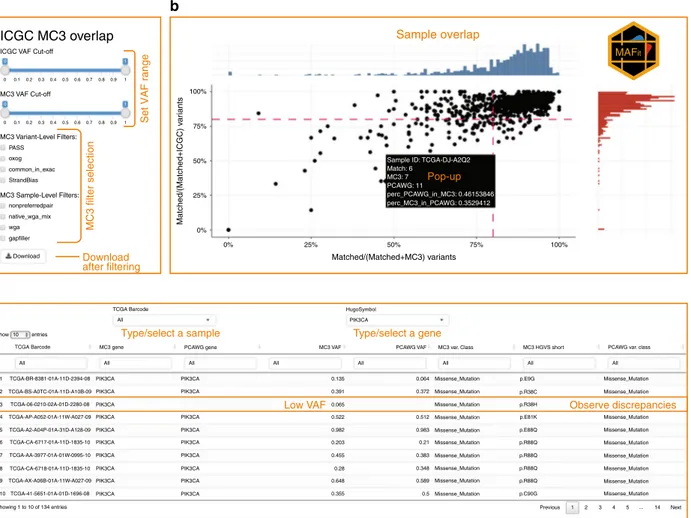
Fig. 3 Recoverability simulation and effects of subclones on mutation concordance. a Observed recovery rate of PCAWG variants in MC3 (red) and of MC3 variants in PCAWG (blue), alongside sequencing noise simulations calculated from random draws of a binomial model that incorporates the VAF and estimated read depth at each site (light red simulates PCAWG recoverability of MC3 variants, and light blue simulated MC3 recoverability of PCAWG

variants).Y-axis is described with legend. X-axis displays VAF of the comparative data set in regard to Y. b A stacked bar chart displays the proportion of

matched and unique variants (y-axis) for different VAF bins (x-axis). 180 variants did not provide read count information and were removed from this

figure. c Stacked proportional histogram shows the fractions of PCAWG matched mutations (purple) and PCAWG-unique mutations (red). Mutations

were restricted to SNVs, and subclonality predictions are indicated as either‘Clonal’ or ‘Sub-clonal’. Columns 2–4 reflect sub-clonal assignment provided

by PCAWG (Note: only a few samples reportedfive predicted subclones and were not included in this analysis). The number of variants represented for

each clonal assignment is shown on the_{x-axis. d Similar to panel c, a stacked proportional histogram illustrates the proportion of matched and unique}

We

investigated

how

many

variants

unique

to

the

MC3 somatic public access call-set could be found in the

PCAWG germline call-set for the same patients. We identified a

total of six such variants (each in a different sample),

five of

which were

flagged in the MC3 public call-set with one filter or

another. Overall, this indicates that variants that have been

incorrectly designated as germline or somatic are an extremely

uncommon source of variation between the two projects.

Variants in GC-extreme intervals. Since it is well-known that the

efficiency of exome capture is adversely affected by very high or

very low GC-content

29,30

_{, we sought to test whether GC-content}

was associated with call rates in MC3 and PCAWG. We used a

plug-in for VEP

31

_{to annotate all matched and private SNVs with}

CADD

32

_{in order to annotate each variant with the percentage of}

the neighboring 100 bases that are a G or C. First, we assessed

how the distribution of read depth across GC-content changes

between MC3 and PCAWG (Fig.

5

b). PCAWG was found to have

a fairly uniform read depth across GC-content bins, while MC3

read depth was concentrated in regions of moderate GC-content

(Fig.

5

c). The low read depth in MC3 at regions of extreme

GC-content was in turn associated with lower variant recovery rates

in these regions but did not grossly affect the number of variants

recovered by MC3 because regions of extreme GC-content are

relatively rare in the genome overall and in exome-capture

regions in particular.

An in-depth analysis of these regions revealed that 76

mutations in known driver genes, identified in the combined

TCGA data by Bailey et al. 2018, were missed in GC poor (GC

fraction < 0.3) or GC rich (GC > 0.7) regions

28

. Three such

instances revealed VHL mutations in KIRC that were overlooked

in GC rich regions of this gene (two of these three recur). In

addition, these 3 samples are not reported to carry a VHL

mutation in the MC3 public data set. Other such instances

include 7 SOX17 mutations, LATS2 (6), and CACNA1A (6). These

findings emphasize the advantages of uniform coverage

using WGS.

The bases

flanking a mutation (tri-nucleotide context) affect

mutation rate, which should be approximately equal between

MC3 and PCAWG, and also the rate of introduction of

sequencing artifacts. Large differences in the call-rates of MC3

and PCAWG and particular nucleotide sequences could indicate

a sequencing artifact unique to one or the other call-set, which

might arise from different procedures for computationally

filtering or biochemically preventing sequencing oxidation

products. Therefore, we sought to test whether the trinucleotide

context of variants correlated with relative call-rates in MC3 and

MC3 filter selection

Set VAF range

Download after filtering

Type/select a sample Type/select a gene

Low VAF Observe discrepancies

Sample overlap Pop-up MAFit

a

b

c

ICGC MC3 overlap

ICGC VAF Cut-off

0 0 1 0 1 0.1 0.2 0.3 0.4 0.5 0.6 0.7 0.8 0.9 1 0 0.1 0.2 0.3 0.4 0.5 0.6 0.7 0.8 0.9 1 MC3 VAF Cut-off PASS 100% 75% 50% 25% 0% 0% PIK3CA 0.135 0.064 p.E9G All All All All All All All All 1 TCGA-BR-8381-01A-11D-2394-08 TCGA-BS-A0TC-01A-11D-A10B-09 TCGA-06-0210-02A-01D-2280-08 TCGA-AP-A052-01A-11W-A027-09 TCGA-A2-A04P-01A-31D-A128-09 TCGA-CA-6717-01A-11D-1835-10 TCGA-AA-3977-01A-01W-0995-10 TCGA-CA-6718-01A-11D-1835-10 TCGA-AX-A06B-01A-11W-A027-09 TCGA-41-5651-01A-01D-1696-08 2 3 4 5 6 7 8 9 10 Showing 1 to 10 of 134 entries Show entries TCGA Barcode TCGA Barcode All

MC3 gene PCAWG gene MC3 VAF PCAWG VAF MC3 var. Class MC3 HGVS short PCAWG var. class PIK3CA HugoSymbol 10 p.R38C p.R38H p.E81K p.E88Q p.R88Q p.R88Q p.R88Q p.R88Q p.C90G Previous 1 2 3 4 5 ... 14 Next Missense_Mutation Missense_Mutation Missense_Mutation Missense_Mutation Missense_Mutation Missense_Mutation Missense_Mutation Missense_Mutation Missense_Mutation Missense_Mutation Missense_Mutation Missense_Mutation Missense_Mutation Missense_Mutation Missense_Mutation Missense_Mutation Missense_Mutation Missense_Mutation Missense_Mutation 0.372 0.512 0.983 0.383 0.348 0.589 0.5 0.21 0.391 0.065 0.522 0.982 0.203 0.455 0.648 0.355 0.28 PIK3CA PIK3CA PIK3CA PIK3CA PIK3CA PIK3CA PIK3CA PIK3CA PIK3CA PIK3CA PIK3CA PIK3CA PIK3CA PIK3CA PIK3CA PIK3CA PIK3CA PIK3CA 25% 50%

Sample ID: TCGA-DJ-A2Q2 Match: 6 MC3: 7 PCAWG: 11 perc_PCAWG_in_MC3: 0.46153846 perc_MC3_in_PCAWG: 0.3529412 Matched/(Matched+MC3) variants Matched/(Matched+ICGC) v a ri ants 75% 100% oxog common_in_exac StrandBias nonpreferredpair native_wga_mix wga gapfiller Download MC3 Variant-Level Filters: MC3 Sample-Level Filters:

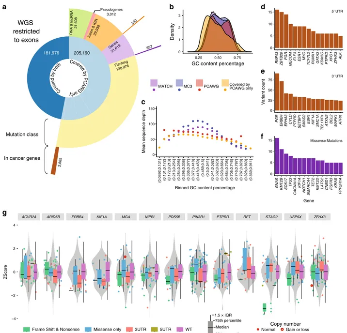
Fig. 4 Screenshots of online tool MAFit. Here we display screenshots from the MAFit on-line interface. Currently there are three main components to

the interface:a A side panel shows sliders and radio buttons tofilter data set to remain inclusive. In addition, a download button is available that will

download the underlying data table.b MAFit rebuilds Fig.2b in the_{first tab of the on-line interface. Each alteration to the radio buttons or VAF sliders will}

result in an updatedfigure. In addition, if one’s hovers over a point on the scatter plot, a pop-up window will automatically display, providing the user with

basic statistics used to calculate that point, i.e., total number of mutations, number of unique and matched mutations.c A table is also presented based on

PCAWG. Before applying the MC3 OxoG

filters, we found a huge

predominance of CA variants unique to MC3, with the

trinucleotide contexts most specific to one database or another

being 7-9 times more specific than the least specific trinucleotide

contexts. After applying the MC3 OxoG

filters, nucleotide

contexts differed by less than four-fold in their specificities. The

residual differential specificity by trinucleotide context after

filtering can either indicate differences in sequencing artifact

abundance and

filtration by project, or could merely be a

consequence of the fact that nucleotide context is also correlated

with VAF and the distance from transcription start sites, which

may independently affect MC3 and PCAWG relative call-rates.

We extended the nucleotide context and performed mutation

spectrum analysis, comparing all MC3 and all PCAWG

mutations found after restricting the two data sets to exonic

regions as described above (Step 3 of Fig.

1

a). We then calculated

ACVR2A ARID5B ERBB4 KIF1A MGA NIPBL PDS5B PIK3R1 PTPRD RET STAG2 USP9X ZFHX3

−4 −2 0 2 4 ZScore 3UTR 5UTR

Frame Shift & Nonsense Missense only WT Median 25th percentile 75th percentile 1.5 × IQR

Copy number

Normal Gain or loss

WGS restricted to exons In cancer genes Mutation class Flanking 128,976 Genes 21,618 Intron & IGR29,938

RNA & lncRNA

21,608 Pseudogenes 3,012 Co ve re d by both Cove red b_y P C A W G onl y 0 5 10 15 GNAS _{KMT2B SOX17} TP53 CACNA1A KIF1A NOTCH1 SMARCA4 TET2 KMT2D LATS2 CNBD1 FGFR3 KRAS PPP2R1A Gene 0 25 50 75 PGR

ERBB4 EPHA3 CYLD PTPRD _SETBP1 SMAD2 ESR1 KIF1A SMC1A

TBL1XR1

ATXN3 BCL2 MAPK1 ATRX

0 5 10 15 RNF43 _ZBTB20 PGR MECOM

ELF3 ESR1 MYC TCF7L2 RUNX1 GA TA3 KDM5C PTPRD XPO1 ZFHX3 ALK Variant count 5’ UTR 3’ UTR Missense Mutations 0 1 2 3 0.25 0.50 0.75 GC content percentage Density

MATCH MC3 PCAWG Covered by_{PCAWG only}

0 50 100 150 (0.0892,0.131] (0.131,0.172] (0.172,0.213] (0.213,0.254] (0.254,0.295] (0.295,0.336] (0.336,0.377] (0.377,0.418] (0.418,0.459] (0.459,0.5] (0.5,0.541] (0.541,0.582] (0.582,0.623] (0.623,0.664] (0.664,0.705] (0.705,0.746] (0.746,0.787] (0.787,0.828] (0.828,0.869] (0.869,0.911]

Binned GC content percentage

Mean sequence depth

181,976 205,190 550 697 2,885

a

b

c

d

e

f

g

Fig. 5 WGS mutations in exonic regions not captured by WES. a A sunburst diagram provides a breakdown of variants that are removed during the

coverage step of the tool. The innermost circle represents the total number of variants identified upon filtering for exome beds used by MC3. Then, we

restrict PCAWG variants to well-covered MC3 regions for each sample. The majority of gencode.v19 annotated and the BROAD target bed_{file of exonic}

regions are sufficiently covered by PCAWG in flanking regions: 3’UTRs, 5’UTR, and 5’Flanking. The outermost ring illustrates the number mutations

identified by PCAWG that were poorly covered by MC3. b A density plot illustrates the density of percent GC-content from a 100 bp window surrounding a

variant. Four variant-sets are displayed: matched, private to MC3, private to PCAWG, and we extend our dataset to include exonic variants not covered by

WES but sufficiently covered in WGS (Covered by PCAWG only). c A scatter plot displays mean sequence depth (y-axis) by increasing GC-content bins

(x-axis). Points are colored according to variant set (same as panel b). d–f Total annotated mutations counts from 3 different annotated regions are shown

for 5UTR, 3UTR, and missense mutations, respectively.g ExpressionZ−Scores for 3’UTR using all TCGA-UCEC samples. Cis-RNAseq expression violin

plots are displayed for 13 genes. On top of the gene-level distribution violin plot, box and whisker plots display sample expression based on mutation

transition and transversion frequencies in each cancer type. After

removing hypermutated samples and OxoG artifacts, we used a

chi-squared test to determine the similarities and differences

between cancer types in the full exome space compared versus the

captured exome space. Strikingly, we did not identify significant

differences in mutation spectrum in the majority of cancers. We

did observe significant differences (FDR < 0.05) in the mutation

spectrum for COAD, KICH, LUAD, and OV (Supplementary

Data 5). These observations included strong discrepancies for AG

and CG transition differences in KICH and OV, respectively. AT

and CA transversions contributed mostly to COAD and LUAD

differences (Supplementary Fig. 9). While these differences may

reflect sequencing artifacts, such as whole genome amplified DNA

in OV or low sample size, we believe the data can still provide

more information pertaining to additional cancer genes and

oncogenic mechanisms.

Non-Coding/Flanking intersections with low coverage. With

the growing use of WGS in many labs, we sought to identify

which mutations are gained by extending to this form of data.

One major observation from our pipeline highlighted that some

variants in exome regions were not well covered by WES (Fig.

1

a

Step 3). Using this mutation set we investigated the most

recur-rent members as derived by WGS but not by MC3 in exonic

regions as defined by gencode.v19 (Fig.

5

a). We observed 697

mutations in cancer genes

28

_{uniquely called by WGS}

(Supple-mentary Data 6). We defined flanking mutations as all

non-translated mutations near exons, i.e., 5’UTR, 3’UTR, 5’Flanking,

and 3’Flanking regions, as they make up the majority of

muta-tions not present in the MC3 public MAF. Recurrent mutation

analysis identified the most frequently mutated genes in 5’UTR

(Fig.

5

d), 3’UTR (Fig.

5

e), and missense mutations (Fig.

5

f). We

found the most frequently mutated 3’UTR in cancer genes was

PGR (91 mutations allowing for multiple mutations per sample),

followed by ERBB4 (72), EPHA3 (42), CYLD (41), and PTPRD

(34). To extend this analysis, we used RNAseq data collected by

TCGA to determine mutation type specific cis-expression

pat-terns, which clearly shows correlation of UTR mutations on RNA

abundance (Fig.

5

g).

Finally, similar to previous studies

33,34

_{, we investigated the}

potential effect of non-coding mutations when determining

significantly mutated genes (SMG). Using MuSiC

35

_{with the}

no-skip-non-coding option, we rescued non-coding mutations

annotated by PCAWG and included them in the significantly

mutated gene (SMG) analysis. We only performed SMG analysis

on cancer types having greater than 35 samples

(BRCA-Breast-AdenoCa, HNSC-Head-SCC, KICH-Kidney-ChRCC,

LIHC-Liver-HCC, LUAD-Lung-AdenoCA, LUSC-Lung-SCC,

SKCM-Skin-Melanoma, STAD-Stomach-AdenoCA,

THCA-Thy-Ade-noCA, and UCEC-Uterus-AdenoCA). We initially identified

potential driver-gene candidates (FUT9, MMP16, SNHG14, and

SFTPB, Fig.

6

) not previously reported in Pan-Cancer whole

genome analysis, but further investigation did not support these

candidates with the exception of SFTPB.

SFTPB (FDR 1.56e−07) in LUAD was recently reported to be

significantly mutated using a larger set of these same data

34

_{. As}

reported, this gene is involved in a lineage-defining surfactant

protein. While six mutations contributed to its SMG status, only 1

3’UTR mutation was reported for LUAD in the MC3 controlled

data set. Furthermore, this single indel was only found by one

variant caller (Varscan). We confirmed the impact of SFTPB UTR

mutations by performing a genome-wide association analysis of

expression differences and found that samples with SFTPB

mutations showed lower RNA abundance in PCDHA7, a gene

known to be involved in cells’ self-recognition and

non-self-discrimination (chi-squared p-value 3.6 × 10

-8

). While other

promising candidates exist, such as FUT9, a fucosyltransferase

involved in organ bud progression during embryogenesis and has

been implicated in cancer initiation

36

, we found no additional

evidence for supporting its driver status.

Discussion

The research community is increasingly leveraging technology

advances to integrate data at larger scales. We performed a

comparative evaluation of ~750 samples with joint exome and

whole genome sequencing mutation calls provided by two

con-sensus mutation calling efforts, MC3 and PCAWG. This joint

data set is encouraging, suggesting that ~80% of the predicted

somatic mutations were captured by both efforts. Furthermore, a

combined 90% of samples have greater than 80% variant

con-cordance when considering covered exonic mutations from

individual cohorts separately. Analysis of this data set also

revealed three major contributors to variant discrepancies: (1) low

variant allele fraction, (2) variant

filtering decisions, and (3)

technological limitations. Software differences were not an

appreciable confounder.

Distinct advantages and disadvantages accompany somatic

mutation calling when utilizing captured WES or WGS. We

found that ~70% of the discrepancies between whole genome and

whole exome sequencing are influenced by low variant allele

fraction. This information holds many implications in identifying

subclonal heterogeneity in the tumor of interest. Other discrepant

calls originate from the decisions made on how to

filter and

distribute publicly available mutation calls. Higher-order

muta-tion signature analysis does not appear to be inordinately affected

by these differences. We show that reported germline variants

were negligible, but nearly 30% of the private PCAWG mutations

were not reported by MC3 because only a single variant detection

algorithm identified them. We want to emphasize that, while

somatic variant detection in cancer is commonplace, there are still

many issues to reconcile.

Finally, we found additional mutations only observable in

exonic regions using either WES or WGS. For example, WES

uniquely identified 424 mutations in cancer genes with median

VAF of ~10%. We also highlight ~700 WGS mutations from

cancer genes, of which ~10% are attributable to regions of high

and low CG-content; thus, highlighting the advantages of more

uniform coverage from WGS.

Only about 2% of the genome is protein coding. For the last

dozen years, cancer genomics has provided a comprehensive

molecular characterization of many different tumor types, thanks

in large part to The Cancer Genome Atlas and other publicly

funded efforts. The community is just starting to explore how

exomics, transcriptomics, proteomics, and methylomics can be

woven together across this 2% of the genome. We anticipate a

general transition from WES to WGS, but this analysis is

meanwhile reassuring that few clerical mutations were overlooked

in WES and that WGS is capable of recapitulating previous

genomic

findings.

Methods

Human research participants. The Cancer Genome Atlas (TCGA) collected both tumor and non-tumor biospecimens from human samples with informed consent

under authorization of local institutional review boards (https://cancergenome.nih.

gov/abouttcga/policies/informedconsent).

Sample overlap. TCGA barcodes carry metadata that reflect tumor portions and

different aliquots. As noted in Fig.1b, TCGA barcode differ slightly in the

com-parison between MC3 and WGS aliquots. A brief description of the breakdown of the TCGA barcode is outlined below.

Example: TCGA-DD-0001-01B-01D-A152 - TCGA-Project

- DD-Tissue source site: the tissue location of tumor that matches clinical metadata.

- 0001-Participant code

- 01-Sample type: i.e., solid tumor (01), primary blood derived tumor (03), solid

tissue normal (11), blood derived normal (10)

- B-Vial: the order in a sequence of samples, i.e., A= first in sequence, B =

second in sequence

- 01-Portion: sequential order of the 100–120 mg of samples

- D-Analyte: molecular analyte type for analysis, i.e., D for DNA and W for WGA.

- A152-Plate: sequential location of a 96-well plate

39% 33% 31% 22% 22% 25% 22% 19% 19% 17% 19% 17% 19% 19% 11% 17% 14% 17% 17% 11% 11% 8% 11% 8% 8% 6% 6% 6% 6% 6% 3% 3% 3% 3% TP53 RYR2 ASXL3 FUT9 MMP16 PTPRD KEAP1 NECAB1 SORCS3 AFF2 CDH12 EGFR KRAS NCAM1 AMER1 PRKCB RBM10 SFTPB STK11 CTNNB1 MET RB1 SOX1 NF1 SMARCA4 ARID1A ATM BRAF MGA SETD2 CDKN2A PIK3CA RIT1 U2AF1 0 5 10 15 0 2 4 6 810 14 27% 18% 22% 22% 12% 12% 10% 10% 10% 10% 8% 8% 8% 6% 8% 8% 6% 6% 6% 6% 6% 6% 4% 4% 4% 4% 4% 2% 2% 2% 2% 2% 2% 2% 2% 2% 0% TP53 ALB CTNNB1 FUT9 AXIN1 BAP1 ARID1A IGF1R SLC6A17 SYT10 AMER1 APOB IDH1 KEAP1 PCDH7 SLITRK1 DHX9 EEF1A1 HMGA2 NES RB1 RPS6KA3 ARID2 CDKN1A IL6ST NRAS XPO1 BRD7 CREB3L3 GNAS KRAS LZTR1 NFE2L2 PIK3CA TSC2 WHSC1 NUP133 0 1 2 3 4 5 6 7 0 2 4 6 810 14 85% 64% 45% 43% 43% 47% 40% 40% 34% 38% 36% 34% 32% 30% 34% 30% 30% 26% 23% 23% 17% 17% 15% 15% 13% 13% 11% 11% 9% 9% 9% 6% 6% 4% 4% 4% 2% 2% 2% TP53 SNHG14 LRP1B NFE2L2 PAPPA2 USH2A FAM135B RYR2 CSMD3 FUT9 MMP16 CDH10 KLHL1 KMT2D NOTCH1 CTNNA2 GREM2 SATB2 CDKN2A SOX11 NF1 FAT1 PIK3CA SLITRK2 CUL3 KDM6A RASA1 SOX1 ARHGAP35 ARID1A FBXW7 PTEN RB1 FGFR2 HRAS KEAP1 EP300 HLA−A KLF5 0 5 10 15 20 0 10 20 30 40 Alterations Lung-SCC Lung-AdenoCA Skin-Melanoma Liver-HCC

CODING INDELS NONCODING

57% 57% 49% 49% 49% 41% 43% 43% 41% 41% 22% 24% 24% 22% 24% 22% 22% 22% 16% 16% 14% 14% 11% 11% 8% 8% 8% 5% 5% 5% 5% 5% 3% 3% GRIN2A FUT9 DSC3 GABRG1 BRAF CADM2 CLEC5A PGR FLG SAMD12 MECOM COL5A1 NF1 NRAS TP53 ARID2 CDKN2A CYLC1 RAC1 DACH1 DDX3X PTEN IDH1 PPP6C CTNNB1 GNA11 KRAS BRD7 CDK4 GYPB KIT RB1 MAP2K1 RQCD1 0 5 10 15 20 25 0 5 10 15 20 25

b

c

d

a

Fig. 6 Significantly mutated gene analysis with the inclusion of UTR mutations. OncoPrint plots were generated using the R package ComplexHeatmap42

for four cancer types: LUAD (a), LIHC (b), LUSC (c), and SKCM (d). We report all SMGs identified by Bailey et al. 201828_{, as well as top significantly}

mutated gene hits from MuSiC that include non-coding mutations. While many non-coding mutations look promising, further investigation yielded little

A lookup table outlining thesefields is located at the GDC:https://gdc.cancer. gov/resources-tcga-users/tcga-code-tables. In order to determine the role of aliquot differences in assessing mutation concordance, we re-analyzed the clonality and overall mutation overlap after stratifying for exact barcode differences. We observed that the effect of matching barcodes on match variant frequency has little effect.

Assessing cancer subtype selection preference. Analysis working groups for TCGA projects were primarily subdivided according to cancer types. Scientific experts gathered in consortia from around the country to participate in char-acterizing many tumors using high throughput data generated on many substrates, e.g., WES, RNAseq, etc. At the conclusion of these projects, groups were asked to hand-select a subset of samples to perform validation sequencing (WGS, the samples used in this analysis). The selection criteria differed from group-to-group and sometimes resulted in an overabundance of one subtype over another. To determine cancer subtype selection bias, we performed an enrichment analysis. Using clinical data we calculated (for each cancer type) the subtype fraction in the WES cancer cohort and measured whether the fraction was similar to WGS set of samples using a Fisher’s exact test.

De_{fining exonic regions. We used the same definition as Ellrott et al. to reduce}

whole genome and exome calls to define genomic coordinates27_.

Coverage calculations. Fixed-step (step= 1) Wiggle coverage files (.wig) for both

MC3 and PCAWG were provided by the Broad Institute. The wig format is a binary readout of sufficient sequencing coverage for genomic data. Here, sufficient coverage is defined as bases with 8 or more reads at a given location. These wig files were processed and reduced to exonic regions using the wig2bed function from

BEDOPTS37_.

After the preliminary screen of coverage-reduced MAFfiles, we observed that

matching mutations (identified by PCAWG and MC3) were removed from one technology and not the other after the coverage reduction step. To account for this issue, we performed a self-coverage reduction step to that identified 6460 mutations. We describe some properties of those mutations here. The median

tumor depth reported by MC3 from these variants is 12 reads (+/− 3 median

absolute difference). The median tumor depth reported by PCAWG in this region is 39 reads (+/− 35.6 median absolute difference), suggesting wide variance of tumor read depths that were removed. However, the mode tumor depth of the PCAWG variants was 13, justifying this removal of variants with low read support. Finally, we determined how many of these poorly-covered variants originated from

cancer driver genes. We observed 126 mutations from the MC3file, and 156 cancer

mutations were eliminated at this stage in the comparison.

Overlapping mutations. After reducing the variants to be within exome sequen-cing target region, within same exon definitions, and having enough sequensequen-cing depth, the remaining variants from ICGC and PCAWG were stored in a SQLite database to enable fast lookup. We then executed a full join between the two sources of variants by matching the donor ID, sample ID, and the genomic range of each variant. The full join output was further cleaned up to remove duplicated filters due to naming variations and duplicated variants due to DNPs.

- Matching IDs - Matching chromosomes

- End position greater than or equal to start position - Start position is less than or equal to end position.

Deduplication of variants. After merging the PCAWG and MC3 data, we observed different strategies were taken by MC3 and PCAWG to capture neigh-boring variants, i.e., complex indels, di-nucleotide (DNP) and tri-nucleotide (TNP) polymorphisms. To address complex indel events (SNVs in indel regions), the MC3 working group absorbed the variants made by SNV callers into the assign-ment made by Pindel. Conversely, PCAWG merged DNP and TNP events into a single event. These strategies resulted in many duplication events from MC3 and PCAWG: 1731 and 62, respectively. These events encompassed 3457 and 119 events, respectively. To address these differences, we merged PCAWG variants into MC3s complex indel events, and MC3 variants into single DNP or TNP events. Filtering optimization. After reducing the starting pool of possible mutations from

746 samples to covered exons, we sought to identify the optimal set of MC3filters

that provide the largest number of samples with greater than 80% concordance from the two technologies with the simplest schema. This was performed

com-prehensively using all possible combinations offilters, often with more than one

filter per variant, with the MC3 cohort (131,071 filter combinations). Filter flags

include:“common_in_exac”, “gapfiller”, “native_wga_mix”, “nonpreferredpair”,

“oxog”, “StrandBias”, and “wga”. We pre-defined the exclusion of variants in MC3 flagged as OxoG along with the inclusion of all PASS variants. The comprehensive filter analysis resulted in two major clusters of variant recoverability (Supple-mentary Fig. 3). Here, we observed the computational trade-off of identifying more

matched variants at the cost of more unique MC3 calls. Below, we highlightfive

strategies considered for analysis (Supplementary Data 2).

1. Only consider variants labeled PASS by the MC3filter column.

2. Only remove variants labeled OxoG by MC3.

3. Prioritize G1 (samples in the most recoverable quadrant, MC3 and PCAWG samples with greater than or equal to 80% from both efforts.)

4. Prioritize total number of matched variants.

5. Maximize total number of samples in the most recoverable quadrant

(Fig.2b) while maximizing the difference between unique MC3 variants and

matched variants thus generating fewer unique calls.

After considering complexity, we chose to move forward with strategy 2 for the

entirety of this study due to its simplicity and relative similarity to otherfiltering

schemes. We recognize that by selecting a singlefiltering strategy, we are limiting

the data slightly and likely introducing some false positive variant calls. However, this strategy allowed us to maintain larger sample sizes and to capture ~15,000 more matched variants than the PASS only strategy at the cost of ~3500 unique mutations calls for MC3.

Assessing mutations per megabase and cancer type concordance. Mutations per megabase data were collected from the broader TCGA dataset and reduced

following the same methods outlined previously28_{. Briefly, this systematically}

removed hypermutators from the dataset. This resulted in a set of 625 samples from the MC3/PCAWG dataset studied here and 8852 TCGA samples. Both Pearson and Mann-Whitney correlations statistics were performed to assess the association of non-silent mutations per megabase and concordance statistics. Simulation of sequencing noise and recoverability. Fan et al. benchmarked the sensitivity of MuSE at recovering somatic variants across 24 combinations of VAF

and read depth3_{. When simulating the recovery of PCAWG variants in MC3 we}

assumed that the VAF observed in PCAWG was the true VAF. We matched the observed VAF of each variant to the closest VAF reported in Fan et al.

For our analysis, the best value to use as the read depth when predicting the MC3 recovery rate of PCAWG variants would be the MC3 read depth at the same site and sample as the PCAWG variant. However, it was not practical to obtain MC3 read depths at sites without MC3 variants, so instead we simulated an MC3 read depth for each PCAWG variant by randomly sampling from the read depths of observed MC3 variants from the same sample as the PCAWG sample. We then matched these simulated read depths for each variant to the closest read depths reported in Fan et al.

For the binned VAFs and read depths for each PCAWG variant obtained as above, we pulled the corresponding sensitivities of MuSE from the Fan et al. paper and simulated MC3 variants with probability equal to these sensitivities. Integrating clonality. Both consortia considered clonality in their comprehensive

characterization of the somatic mutations. Locations of thesefiles are provided in

the data availability section. Here, we provide a brief summary of the strategies used to compile these resources. First, the PanCancer Atlas working-groups used

MC3 mutations to predict subclonal structures using ABSOLUTE38_{. This tool uses}

copy number, recurrent karyotype, and mutation data to calculate copy number purity and cluster identification. Furthermore, the PanCancer Atlas working group only made the distinction of clonal and subclonal mutations and did not attempt to further assign sub-clonal mutations to other likely heterogeneous clusters. PCAWG, on the other hand, used a consensus calling approach incorporating 11 different clustering tools. Here, we evaluated cluster-ID which represents those

mutations that are clonal (ID= 1), with other clusters representing mutations that

are subclonal (ID= 2 through 4). For this analysis, we restricted our data to SNVs

to be consistent with calls made by the PanCancer Atlas calls of MC3 mutations. Fraction of private variation explained. In Supplementary Fig. 7 we provide a breakdown of different sources of variant described in our analysis using publicly available data. For MC3 all private variants were classified as into 3 variant types (Indel, MissensePlus, and Other). Specifically, indels are comprised of:

“Frame_-Shift_Del”, “In_Frame_Ins”, “Frame_Shift_Ins”, and “In_Frame_Del”. MissensePlus

variants are comprised of:“Missense_Mutation”, “Nonsense_Mutation”,

“Non-stop_Mutation”, “Splice_Site”. And Other variants are comprised of: “RNA”, “3’UTR”, “5’UTR”, “5’Flank”, “Silent”, “3’Flank”, “Intron”, “Translation_Start_Site”.

On the other hand, PCAWG variants were also categorized into Indels, MissensePlus, and Other. Specifically, indels are comprised of: “Frame_Shift_Del”, “Frame_Shift_Ins”, “De_novo_Start_InFrame”, “Start_Codon_Ins”,

“Stop_Codon_Ins”, “In_Frame_Del”, “In_Frame_Ins”, “Stop_Codon_Del”, and “Start_Codon_Del”. MissensePlus variants are comprised of: “Missense_Mutation”, “Nonsense_Mutation”, “Nonstop_Mutation”, “Splice_Site”. And other variants are

comprised of:“5’UTR”, “RNA”, “5’Flank”, “Silent”, “3’UTR”, “Intron”, “IGR”,

“lincRNA”, “De_novo_Start_OutOfFrame”, and “Start_Codon_SNP”. In addition to the three variant type categories, six additional sources of variation were added to private variants: Subclonal, VAF5, VAF10, MMcomplement, THCA KICH or PRAD, and GCcontents. As mentioned, subclonal variants are tagged if labeled as identified by the TCGA or ICGC