Numerical Simulation of Flow Field and Organism Concentration in a UV
Disinfection Channel
LI Chan
+, DENG Baoqing
*, Kim Chang Nyung
**Key Words: UV disinfection channel; CFD; Numerical model
Abstract
This paper investigates the flow field and organism concentration in a UV disinfection channel in which vertical ultraviolet lamps are arranged in a staggered configuration. Turbulence is described by low Reynolds number k-ε turbulence model and standard k-ε turbulence model, respectively. P-1 method has been employed to solve the radiative transfer equation. The obtained incident radiation is used to compute the inactivation term in the species equation. The CFD results are in good agreement with the existing experimental data for the UV channel. For the flow field, the low-Reynolds number k-ε model is superior to the standard k-ε model. The approach velocity has a significant effect on the disinfection efficiency. The organism concentration at the outlet decreases fast to a low inlet velocity.
1. Introduction
Coliforms bacteria have a significant influence on human health in drinking water. Some methods have been presented to remove coliforms from water, such as, chlorine, ozonation, microfiltration and UV light (Murphy et al. 2008; Paraskeya and Graham 2005; Watts et al. 1995). Thereinto, the UV disinfection is a widely used method because of its high disinfection efficiency and no secondary pollution. In order to optimize performance or get reliable prediction for control, numerical simulation of flow and species transport in the
UV reactor is necessary.
Recently numerical simulations used by computational fluid dynamics (CFD) have been paid much attention to. Sozzi and Taghipour (2006) investigated the flow field of annular photo-reactor by high Reynolds number k-ε model, Realizable k-ε model and Reynolds stress model. Lyn and Chiu (1999) employed the high Reynolds number k-ε model to calculate the flow field. A good agreement between predictions and measurements has been reported in the results for the velocity, but a striking disparity has been observed for the kinetic energy. Rauen et al. (2008) performed CFD simulation using a low-Reynolds number k-ε model to account for turbulence levels in baffled chlorine contact tanks. Good agreement was obtained for the assessed flow features.
In the UV disinfection, UV light kills the bacteria. So the distribution of UV intensity is important for the optimization of reactor. Blatchley (1997) optimized a design of collimator by use of the line source integration. Chiu and Lyn (1999) employed the point source method
+
Department of Mechanical Engineering, Kyung Hee University, Yongin, 446-701, Korea
*College of Urban Construction and Environmental Engineering, University of Shanghai for Science and Technology, Shanghai 200093, People’s Republic of China
**College of Advanced Technology, Kyung Hee University, Yongin, 446-701, Korea
E-mail: [email protected]
to obtain the intensity field of a whole UV channel. Lyn and Chui (1999) also used the point-source summation technique as an integral over the length of a UV lamp. Pareek and Adesina (2004) used a discrete ordinate model to solve the RTE. It can easily predict light intensity in more complex reactor geometries.
Ducoste (2005) used the Lagrangian and Eulerian methods to model the microbial inactivation. The results showed the Eulerian approach seemed comparable to the Lagrangian particle tracking approach. In these literatures, the calculations of flow field have not been accurate and the calculated UV intensities have been unreasonable, which has resulted in the underestimate or overestimate of the disinfection efficiency.
In the present study, the low-Re number k-ε turbulence model and Standard k-ε turbulence model are used to calculate the flow field. The P-1 model is employed to obtain the intensity field. The species equation is applied to compute the inactivation of organism. Numerical results are compared with experimental measurements in a laboratory-scale UV system.
2. Integrated UV disinfection model
UV disinfection concerns the flow of water in the reactor, the distribution of UV light in the reactor and the inactivation of bacteria. The performance of the reactor depends on the interaction of these three parts.2.1 Flow modeling
The flow in the reactor not only has a strong influence on the microorganism distribution but also can affect the efficiency of disinfection. Therefore, it is necessary to predict the flow field in the UV channel accurately. The flow in the reactor can be described by Navies-Stokes equations. Based on the eddy-viscosity approximation, the governing equations can be written as follows;
( )
j 0 j u x r r t ¶ ¶ + = ¶ ¶ (1)( )
i(
i j)
j i i j i j j u u u x p u u u x x x r r t rn r ¶ ¶ + ¶ ¶ ¶ ¶ ¶ ¢ ¢ = - + -¶ ¶ ¶æ
ö
ç
÷
è
ø
(2) 2 3 j i i j t ij j i u u u u k x x n ¶ ¶ d ¢ ¢ - = + -¶ ¶æ
ö
ç
÷
è
ø
(3) 2 t k C fm m n e = (4)where ν and νt are laminar and turbulent kinematic
viscosities, respectively. The latter one should be determined by a suitable turbulence model. In the present study, the low-Re number k-ε turbulence model is used to determine the turbulent kinematic viscosity. The governing equations of the turbulent kinetic energy k and its dissipation rate ε are written as follows;
( )
(
)
(
)
j j t k k j j k u k x k G x x r r t r n n s re ¶ ¶ + ¶ ¶ ¶ ¶ = + + -¶ ¶é
ù
ê
ú
ë
û
(5)( )
(
)
(
)
1 2 2 j j t k j j u x C G C f x e x e k e e k re r e t e e e r n n s r ¶ ¶ + ¶ ¶ ¶ ¶ = + + -¶ ¶é
ù
ê
ú
ë
û
(6)(
)
{
}
2 2 *14 0.75 200 1 e 15
t e t R y fm R æ ö÷ ç -ç ÷÷ - - çè ÷ø = - +é
ù
ê
ú
ê
ú
ê
ú
ë
û
(7)(
*3.1)
2 ( )2 6.5 1 0.3e1 e
y Rt fe =é
ê
-
-ù é
ú ë
´ - -ù
û
ë
û
(8)The model constants are given by Abe et al. (1994) as follows;
0.09
Cm = ,s =k 1.4,s =e 1.4,Ce1=1.5,Ce2 =1.9.
2.2 Radiation modeling
distribution in a UV channel. The transport equation for the incident radiation G can be written as follows;
( G) aG 0
Ñ × GÑ - = (9)
where Г is the diffusion coefficient of G (m) described by Eq. (10), a is the absorption coefficient (m-1).
1 3(a ss) Css G =
+ - (10)
In the reactor, UV light is emitted from UV lamp. However, the UV distribution in the space of UV lamp is of little importance. So a light source model is needed to describe the UV light intensity from the UV lamp into the reactor. A model for G incorporating the effects of absorption by the quartz tubing and the fluid continuum is obtained using the line-source-integration technique (Pareek and Adesina 2004).
( ) 2 2 2 2 2 2 1 2 1 e 4 l i l w D r qt r r z S G dz L r z a a p -é ù -ë - + û + = +
ò
(11)where S is the lamp output power; l is the length of the lamp; r the distance between a point (x,y) and a single lamp centered (0,0); z the vertical coordinate; αw and αq
absorption coefficient of radiation in water and in quartz tubing, respectively; t the thickness of the quartz jacket.
Integration on Eq. (11) yields the intensity on the surface of the lamp.
(
)
( ) 2 2 2 2 2 2 1 e 4 l l q t r R z S G dz L R z a p -- + = +ò
(12)2.3 Species equation
The transport of microorganisms in the reactor can be described by a convection-diffusion equation.
( )
(
j)
j t j c j C u C x C S x Sc x r r t n n r r s ¶ ¶ + ¶ ¶ ¶ ¶ = + + ¶ ¶é
æ
ö
ù
ê
ç
è
÷
ø
ú
ë
û
(13)where C is the microorganism concentration; r is the reaction rate; K is an intrinsic rate constant;G is the
incident radiation (W-m-2). S represents the inactivation of microorganism due to UV light. For simplicity, it can be described Chick-Waston Law.
S= -KGC (14)
where K is an intrinsic rate constant.
2.4 Boundary condition and initial condition
The flow equations must be complemented by setting boundary conditions. At the inlet, the uniform unidirectional initial velocity (U) is imposed. Turbulent intensity and turbulent length scale are set to 3.8 % and 2.5 cm, respectively. At the outlet, the gradient of all variables are set to zero. At all walls, no-slip boundary condition and wall function are used for velocity and turbulence, respectively. The gradient of the concentration at the wall is also set to zero, but the value of intensity is set by UDF. On the lateral boundaries (excepting the solid boundaries), a symmetry condition is imposed, so that there is no flux across them.3. Geometry of the structure
The physical model has 25 cylindrical UV lamps, each with a diameter of 2.5 cm. Lamps are arranged in five rows, with five lamps in each row, in a staggered configuration. In the numerical simulation, to keep high spatial resolution at reasonable computational effort, only a central region rather than entire flow region is investigated. The modeled region is 33D long and 1.5D wide. The first lamp is 5.5D away from the entrance, and the distance of each two adjacent tubes is 5D.
4. Numerical procedure
The finite-volume method is adopted to solve two-dimensional governing equations. The two-dimensional channel model is divided into 97767 and 50866 triangular grids for the low-Re k-ε turbulence model and the Standard k-ε turbulence model, respectively. The finer grid is set near the UV lamps to
account for the turbulence. The commercial software FLUENT 6.3 is used to solve the continuity, velocity and turbulence equations. Turbulence is described by low Reynolds number k-ε turbulence model and Standard k-ε turbulence model, respectively. P-1 method has been employed to solve the radiative transfer equation. The obtained incident radiation is used to compute the inactivation term in the species equation.
5. Results and discussions
The parameters used in this paper are as follows; The value of S/L is 26.7 W over a 1.47-m arc; l is 0.74 m; the values of αw and αq are 44 m-1 and 63 m-1,respectively; t is 1.5×10⁻³ m; R is 0.0125 m; K is 0.059 m2W-1s-1.
5.1 Results of flow field
The mean streamwise velocities u/U and the mean transverse velocities v/U obtained by the low-Re number k-ε turbulence model and the Standard k-ε turbulence model are shown in Fig. 1 and 2. The values of u/U after each lamp are negative meaning that the back flow is generated inside these regions. For v/U, although a slight disparity between predictions and measurements is observed, their variety trends are similar.
The normalized kinetic energy k/U2 obtained by the simulation and experiment are depicted in Fig. 3. A big disagreement between the numerical and experimental results is observed for the turbulent kinetic energy k/U2.
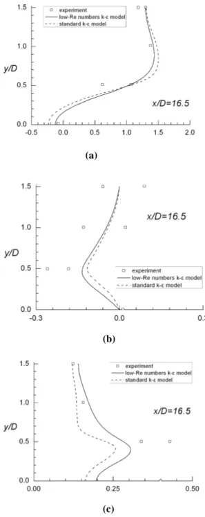
Fig. 4(a) shows the comparison of the mean streamwise velocities obtained by the simulation and experimental results at various x/D sections. The predictions of u/U are rather good. Although the measured v/U profiles exhibit large scatter, the numerical results are often within the scatter of the measurements. Large discrepancies between measurements and predictions of k/U2 seen in Fig. 4(c) are also found on the results of Lyn’s paper (Lyn et al. 1999).
5.2 Results of disinfection simulation
Fig. 5 shows the computed intensity field. The intensity between each two adjacent lamps is very low, so that the effect of other lamps can be neglected.Fig. 6 depicts the organism concentration in the channel when the approach velocity is 0.15 m/s.
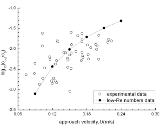
Fig. 7 illustrates the comparison of measured and predicted concentration at the outlet with the different approach velocities. The figure shows when the approach velocity is lower, the disinfection efficiency is higher. This is because the retention time increases with the decrease of the approach velocity. Then, the organisms have much opportunity to absorb UV light.
6. Conclusion
This paper investigates the flow field and organism concentration of a UV disinfection channel in which vertical ultraviolet lamps are arranged in a staggered configuration. The commercial software FLUENT 6.3 has been employed to solve the continuity, velocity and turbulence equations. For the flow field, the low-Reynolds number k-ε model is somewhat superior to the Standard k-ε model. The disinfection efficiency had a significant variety with the change of inlet velocity. The organism concentration at the outlet decreased fast to a low inlet velocity. Overall, the CFD modeling results were in good agreement with the experimental data for the UV disinfection channel. All numerical results are more similar to the experimental data than those from any other papers related to the UV disinfection channel. These verified CFD models could represent the flow structure for an UV disinfection channel and could be used for UV channel performance simulation.
Figures
Fig. 1 The mean streamwise velocities along the line of y/D = 0
Fig. 2 The longitudinal profile of mean transverse velocities along the line of y/D = 0.5
Fig. 3 The longitudinal profile of normalized kinetic energy along the line of y/D = 0
Fig. 4 The comparison among the low-Re number and the Standard k-ε model and experimental results along four lines: (a) the mean streamwise velocities, (b) the mean transverse velocities, (c) the normalized kinetic energy
(b)
(c) (a)
Fig. 5 The UV intensity field of the disinfection channel (out of scale)
Fig. 6 The concentration field of the disinfection channel when the different approach velocity is 0.15 m/s (out of scale)
Fig. 7 Comparison of measured and predicted log10(cout/c0) as function of approach velocity
References
(1) Abe, K., Kondoh, T., and Nagano, Y., 1994,
"A new turbulence model for predicting fluid flow and heat transfer in separating and reattaching flows–I. Flow field calculations." International Journal of Heat and Mass Transfer, Vol. 38, No. 8, pp. 139~151.
(2) Blatchley, E. R., 1997, "Numerical modelling of UV intensity: Application to collimated-beam reactors and continuous-flow systems."Water Research, Vol. 31, No. 9, pp. 2205~2218.
(3) Chiu, K., Lyn, D. A., Savoye, P., and
Blatchley III, E. R., 1999, "Integrated UV Disinfection Model Based on Particle Tracking." J. Environ. Eng. Vol. 125, No. 1, pp. 7~16.
(4) Ducoste, J. J., Liu, D., and Linden, K., 2005,
"Alternative Approaches to Modeling Fluence Distribution and Microbial Inactivation in Ultraviolet Reactors: Lagrangian versus Eulerian." J. Environ. Eng. ASCE, Vol. 131, No. 10, pp. 1393~1403.
(5) Lyn, D. A., Chiu, K., and Blatchley, E. R. I.,
1999, "Numerical Modeling of Flow and Disinfection in UV Disinfection Channels." J. Environ. Eng. ASCE, Vol. 125, No. 17, pp. 17~26.
(6) Murphy, H. M., Payne, S. J., and Gagnon, G.
A., 2008, "Sequential UV-and chlorine-based disinfection to mitigate Escherichia coli in drinking water biofilms." Water Research, Vol. 42, No. 8~9, pp. 2083~2092.
(7) Paraskeva, P., and Graham, N. J. D., 2005,
"Treatment of a secondary municipal effluent by ozone, UV and microfiltration: microbial reduction and effect on effluent quality." Desalination, Vol. 186, No. 1~3, pp. 47~56.
(8) Pareek, V. K., and Adesina, A. A., 2004,
"Light intensity distribution in a photocatalytic reactor using finite volume." AIChE Journal, Vol. 50, No. 6, pp. 1273~1288.
(9) Rauen, W. B., Lin, B., Falconer, R. A., and
Teixeira, E. C., 2008, "CFD and experimental model studies for water disinfection tanks with low Reynolds number flows." Chemical
Engineering Journal, Vol.137, No. 3, pp. 550~560.
(10) Sozzi, D. A., and Taghipour, F., 2006,
"Computational and experimental study of annular photo-reactor hydrodynamics." International Journal of Heat and Fluid Flow, Vol. 27, No. 6, pp. 1043~1053.
(11) Watts, R. J., Kong, S., Orr, M. P., Miller, G.
C., and Henry, B. E., 1995, "Photocatalytic inactivation of coliform bacteria and viruses in secondary wastewater effluent." Water Research, Vol. 29, No. 1, pp. 95~100.