Two Dimensional CFD Analyses on the Heat Transfer for a Supercritical Pressure CO
2Bong Hyun Cho, Young In Kim, andYoon Yeong Bae
Korea Atomic Energy Research Institute, 150 Deokjin-dong Yuseong-gu, Daejeon 305-353, Korea, [email protected]
1. Introduction
The Supercritical Water Cooled Reactor(SCWR) operates in a pressure around 25MPa and temperature of 293~510℃. In order to study the heat transfer behaviors and good comparisons between the various fluids, a heat transfer test loop(SPHINX) using CO2 has been
constructed in KAERI as a part of international research program, I-NERI. At a supercritical pressure, the heat transfer coefficient is much larger than that estimated from the Dittus-Boelter correlation for a relatively large flow rate with moderate wall heat flux conditions.[1] This phenomenon was explained by the rapid variations of the physical properties near the wall with the temperature. On the contrary, the heat transfer becomes worse when the bulk fluid enthalpy is below the pseudo-critical enthalpy under a low flow rate with large heat flux conditions. This phenomenon is called ‘deteriorated heat transfer’, and which is explained as the modification of the shear stress distribution across the tube to a buoyancy and/or acceleration in a low density layer near the wall, with the consequence of a turbulence.[2]The upward vertical flow of CO2 through a uniformly heated tube of 4.4 mm in
diameter and 3m long(heated length is 2.1m) was investigated numerically using the CFD code, FLUENT. Through the numerical simulations, we have attempted to obtain a physically meaningful insight into the heat transfer mechanisms at a supercritical pressure.
2. Numerical Models
We deal with the steady state and 2D-axisymmetric flow field for simplicity. The selected turbulence models for this study are the RNG k-ε(RNG) model with an enhanced wall treatment and the low-Reynolds number Abid(ABID) model. The RNG model is known to estimate more correctly the flow field with rapid strain rates and streamline curvatures than the SKE model does. The low-Reynolds k-ε model has complex damping functions, which permit the integration of the turbulence transport equations over the viscous sub-layer.
The two-layer approach in FLUENT, which is used in this study for the high-Reynolds models, specifies both the dissipation rate and the turbulent viscosity in the near-wall cells.[3] In this approach, the whole domain is subdivided into a viscosity-affected region and a fully-turbulent region, which is determined by a wall-distance-based, turbulent Reynolds number(Rey). In the fully-turbulent
region(Rey>200), the k-ε models are employed. In the
viscosity-affected region(Rey<200), the one equation
model of Wolfstein[4], where the momentum equations and the k equation are retained but the turbulent viscosity
t
µ
is computed from;µt,2layer=ρCµlµ k , lµ: length scale (1)
In the enhanced wall treatment, the turbulent viscosity is smoothly blended with the high-Reynolds number
t
µdefinition from the outer region.
layer t t enh t,
λ
µ
(1λ
)µ
,2µ
= ε + − ε (2)The blending function
λ
εis defined in such a way that it is equal to unity far from the walls and is zero very near the walls. If the near-wall mesh is fine enough to be able to solve the laminar sub-layer(typically +≈1y ), then the enhanced wall treatment will be identical to a two layer zonal model. The sensitivity of the near wall mesh size was tested by earlier studies. Roelofs[5] also recommends a +
y value from 0.1 up to 1 for RNG model through their sensitivity studies.
Since the low-Reynolds turbulence models require that the first grid off the wall has a height of y1 <1
+ , the ABID
model also have a fine grid at the wall. In our numerical simulation, the nearest grid is sufficiently fine everywhere as y1 <1
+ for both models, and the aspect ratio of the grid
becomes very large.
3. Results and Discussions
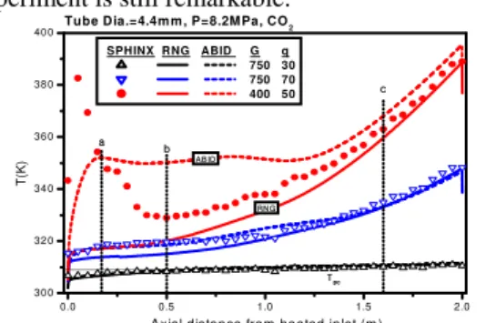
The predicted wall temperatures based on the RNG and ABID model are compared with the measurement in Figure 1. In a normal heat transfer condition with a low heat flux(750kg/m2⋅s, 30kW/m2), the wall temperature
predicted by the RNG and ABID model are very close to the measurement through the entire range of the tube length, but the ABID model seems to predict the more accurately than the RNG does. For the heat fluxes over 70kW/m2, the RNG model shows a fairly large under-prediction at the first half of the tube length, while the ABID model follows the prediction fairly well. In a deterioration heat transfer condition, where the mass flux is 400kg/m2⋅s and the wall heat flux 50kW/m2, both models do not reproduce the experiment well. But the prediction by the ABID model quickly reaches a high temperature just after the entrance region and remains there up to a good distance from the inlet. In the
Transactions of the Korean Nuclear Society Autumn Meeting Busan, Korea, October 27-28, 2005
downstream region the difference between this model and the experiment is still remarkable.
0.0 0.5 1.0 1.5 2.0 30 0 32 0 34 0 36 0 38 0
40 0 Tube Dia.=4.4m m , P=8.2M Pa, CO2
Tpc c b a RNG AB ID SPHINX RNG ABID G q 750 30 750 70 400 50
A xial distan ce from he ated in let (m )
T
(K
)
Figure 1 Predicted wall temperature with measurements for several wall heat fluxes
In order to evaluate the radial-direction flow distribution at the tube axial locations, reference cross-sections are selected as shown in Figure 1(a, b and c). The location of ‘a’ and ‘b’ are selected for the place where
w
T >Tpc>T when q=50-70kW/mb 2 and
pc
T >T >w T when b q=30kW/m2. The location of ‘c’ is selected where
w
T >T >b Tpcfor all the cases. Figure 2 shows the profiles of
the axial velocity and the normalized density. In a normal heat transfer condition[refer to Figure 2 (a) and (b)], the predicted velocities by the two models are barely distinguishable for both heat fluxes. On the contrary, the density profiles for the heat flux 70kW/m2, especially at the location of ‘b’, show remarkable differences between the two models. This may explain the favorable prediction capability of the ABID model under the condition of heat flux of 70kW/m2 in Figure 1. As the fluid travels downstream, the bulk velocity increases because of the density decrease. In a deterioration heat transfer condition[Figure 2 (c)], the predicted velocities by the two models show almost no differences, but the density profiles, especially at the location of ‘b’, shows large differences between the two models. This explains the different trend of the wall temperature prediction shown in Figure 1. The density is drastically decreased for the ABID model at a very near wall region. The degree of spreading is more significant for the ABID model than the RNG model. This may be the cause of the plateau shown by the ABID model in Figure 1. One of the mechanisms of heat transfer deterioration can be explained as flow acceleration by the density variation. The flow near the pseudo-critical point experiences a rapid acceleration when a strong wall heat flux is applied.
4. Conclusion
The numerical prediction has been confirmed to give reasonable information for establishing the experiment. In a normal heat transfer condition with a low heat flux, both the RNG with an enhanced wall treatment and the ABID
model predict well the experiment. But in a relatively large heat flux condition, the ABID model predicts the experiment better than the RNG model. In a deteriorated heat transfer conditions, the ABID model prediction shows a localized temperature plateau a good distance away from the entrance region, and the difference between this model and the experiment is remarkable. Through the examination of the radial distribution of the fluid properties, a part of the reason for the heat transfer deterioration mechanism is a broadening of a region of a low density and the low specific heat off the wall.
0 . 8 0 0 . 8 5 0 . 9 0 0 . 9 5 1 . 0 0 0 . 0 0 . 5 1 . 0 1 . 5 2 . 0 2 . 5 3 . 0 0 . 5 1 . 0 1 . 5 D e n s i t y A x i a l V e l o c i t y r / R ρ / ρ(p c) Ux ( m /s ) a b c B l a n k S y m b o l : R N G F i l l e d S y m b o l : A B I D T u b e D i a . = 4 . 4 m m , P = 8 . 2 M P a , C O2 G = 7 5 0 k g / m2s , q = 3 0 k W / m2 (a) 0 . 8 0 0 . 8 5 0 . 9 0 0 . 9 5 1 . 0 0 0 . 0 0 . 5 1 . 0 1 . 5 2 . 0 2 . 5 3 . 0 0 . 5 1 . 0 1 . 5 D e n s i t y A x i a l V e l o c i t y r / R Ux ( m /s ) ρ / ρ(pc) a b c B l a n k S y m b o l : R N G F i l l e d S y m b o l : A B I D T u b e D i a . = 4 . 4 m m , P = 8 . 2 M P a , C O2 G = 7 5 0 k g / m2s , q = 7 0 k W / m2 (b) 0 . 8 0 0 . 8 5 0 . 9 0 0 . 9 5 1 . 0 0 0 . 0 0 . 5 1 . 0 1 . 5 2 . 0 2 . 5 3 . 0 0 . 5 1 . 0 1 . 5 r / R Ux ( m /s ) ρ / ρ(p c) D e n s i t y A x i a l V e l o c i t y a b c B l a n k S y m b o l : R N G F i l l e d S y m b o l : A B I D T u b e D i a . = 4 . 4 m m , P = 8 . 2 M P a , C O2 G = 4 0 0 k g / m2s , q = 5 0 k W / m2 (c) Figure 2 Predicted axial velocity and density profiles in a radial coordinates
REFERENCES
[1] S. Yoshida and H. Mori, “Heat transfer to supercritical fluids flowing in tubes,” SCR-2000, The University of Tokyo, Nov. 6-9, pp. 72-78, 2000.
[2] W.B Hall and J. D. Jackson, “Laminarlisation of a turbulent pipe flow by buoyancy forces,” ASME Paper No. 69-HT-55, 1969.
[3] Fluent 6.2 User’s Guide, 2004.
[4] M. Wolfstein, “The velocity and temperature distribution of one-dimensional flow with turbulence augmentation and pressure gradient,” Int. J. Heat Mass Transfer, 12: pp.301-318, 1969.
[5] F. Roelofs and and E. Komen, “Heat transfer to supercritical water in SCWR relevant geometry,” ENC 2005, Abstract no. 113, Versailles, December 11-14, 2005.