2344
Copyright ⓒ The Korean Institute of Electrical Engineers
A Coupled Recursive Total Least Squares-Based Online Parameter
Estimation for PMSM
Yangding Wang*, Shen Xu
†, Hai Huang**, Yiping Guo* and Hai Jin**
Abstract
– A coupled recursive total least squares (CRTLS) algorithm is proposed for parameter estimation of permanent magnet synchronous machines (PMSMs). TLS considers the errors of both input variables and output ones, and thus achieves more accurate estimates than standard least squares method does. The proposed algorithm consists of two recursive total least squares (RTLS) algorithms for the d-axis subsystem and q-axis subsystem respectively. The incremental singular value decomposition (SVD) for the RTLS obtained by an approximate calculation with less computation. The performance of the CRTLS is demonstrated by simulation and experimental results.Keywords:
Online parameter estimation, Permanent magnet synchronous machine (PMSM), Total least squares (TLS), Singular value decomposition (SVD).1. Introduction
Permanent magnet synchronous machines (PMSMs) are widely used in industrial servo drives, robotics, electric vehicles and wind power generators etc., due to their high efficiency, high power density, good control performance, simple structure and reliable operation [1]. It is important to obtain accurate knowledge of PMSM parameters for online condition monitoring, fault diagnosis and high-performance control system design.
Many methods have been presented to estimate PMSM parameters, which can be classified into offline methods and online ones. Some offline methods keep the machine at standstill state and inject signals of current or voltage. For example, a dc step voltage [2] was injected into the PMSM at standstill to estimate stator resistance and dq axis inductances. The standstill frequency-response (SSFR) test [3], which evaluates the responses with a sequence of sinusoidal signal injection, is an attractive method to estimate the machine parameters with the drawback of the requirement for special equipment. However, there are some drawbacks for the offline methods. These methods usually require additional measurement instruments and operations to keep the machine at standstill. More importantly, the machine parameters of PMSM vary with temperature change, magnetic saturation and demagnetiza-tion of rotors during the practical applicademagnetiza-tions.
In order to overcome these shortcomings, the online methods update the estimated parameters in real time. Several online methods such as recursive least squares
(RLS) [4, 5], extended Kalman filter (EKF) [6], model reference adaptive system (MRAS) [7], neural network (NN) [8] and particle swarm optimization (PSO) [9] et al. have been proposed. RLS algorithm has been widely used to estimate PMSM parameters for its simplicity and universal application. But the results generated by RLS are easy to suffer from the noise interference. In [6], dq axis inductances estimated by EKF were used to improve the performance of maximum torque per ampere (MTPA) control. In the MRAS method [7], one parameter was estimated by setting the other parameters to be their nominal values. In [8], an adaline NN was used to estimate rotor flux linkage and stator resistance according to rotor position offsets. In [9], a PSO with learning strategy was proposed to estimate PMSM parameters. In addition, the parameters were estimated by two affine projection algorithms according to the parameter dynamics [10].
The method of Total least squares (TLS) is an improved standard least squares method by considering the errors of input variables and output variables at the same time. TLS has been employed to adaptive filtering [11] and parameter estimation for a number of different applications [12, 13]. The problem of TLS is usually solved by the singular value decomposition (SVD). The recursive TLS (RTLS) [14, 15] is required for the online application.
This paper proposes a coupled recursive total least squares (CRTLS) algorithm to estimate PMSM parameters online. The algorithm decomposes the problem into d-axis and q-axis subsystem, performs recursive TLS for each subsystem and couples the results of the two subsystems. In the recursive TLS, the incremental SVD is achieved by an approximate calculation with less computation [15]. Simulations and experiments are performed to verify the effectiveness of the proposed algorithm.
This paper is organized as follows. The model of PMSM and the method of RLS are described in Section 2. The
† Corresponding Author: College of Electrical Engineering, Zhejiang University, China. ([email protected])
* Ningbo Academy of Product Quality Supervision & Inspection, China. ([email protected], [email protected])
** School of Information and Technology, Zhejiang Sci-Tech University, China. ([email protected], [email protected]) Received: December 4, 2017; Accepted: July 17, 2018
CRTLS algorithm is proposed in Section 3. Simulation and experimental results are given in Section 4.
2. PMSM Model and RLS Algorithm for
Parameter Estimation
2.1 PMSM model
Assuming that the PMSM has negligible cross-coupling magnetic saturation, structural asymmetry, iron losses, magnet eddy current loss, and rotor anisotropy, the model of PMSM in the synchronous rotating reference frame is shown as follows: s s d d d d q q e q q q q d d e e m di u R i L L i dt di u R i L L i dt ì = + -ï ï í ï = + + + ï î w w w l (1)
where ud, uq and id, iq are the d-axis and q-axis voltages and currents, respectively. Rs is the stator winding resistance. Ld and Lqare the equivalent d-axis and q-axis inductances, respectively. λmis the permanent magnet flux linkage. ωe is the electrical angular speed.
The measured stator currents for machine control ia, ib and ic are phase variables with stationary reference frame.
id and iq can be computed by the following formulation:
T T T d q a b c i i M i i i é ù = éë ùû ë û (2) cos sin 2 cos( 2 / 3) sin( 2 / 3) 3 cos( 2 / 3) sin( 2 / 3) e e e e e e M -é ù ê ú = - - -ê + - + ú ë û q q q p q p q p q p (3)
The four parameters to be estimated are the stator resistance Rs, the PM flux linkage λm, and the model inductances Ld and Lq.
2.2 The method of least squares
The least squares (LS) algorithm has been widely applied into parameter estimation and system modeling due to its simplicity and universal application. A discrete-time system of PMSM can be modeled as
) ( ) ( ) (k hk e k y =
q
+ (4) where T ( ) d( ) q( ) y k = ëéu k u k ù û (5)[
]
T s Ld Lq m Rl
q
= (6) ' ' ( ) ( ) ( ) ( ) 0 ( ) ( ) ( ) ( ) ( ) ( ) d d q q d q i k i k k i k h k i k k i k i k k é - ù = ê ú ê ú ë û w w w (7)where the discrete-time k = 0, 1, 2, … and y(k) is system output. h(k) is the measured data vector, and q is the unknown model parameter vector. e(k) is a noise term.
For L samples, there are the following equations:
L L y =Hq+e (8) where T [ (1), (2), , ( )] L y = y y K y L (9) T [ (1), (2), , ( )] H= h h K h L (10) T [ (1), (2), , ( )] L e = e e K e L (11)
In most variants of least squares algorithms, the following criterion function is defined and minimized:
2 : ( ( ) ( ) )
k
J =
å
y k -h kq (12)The estimated vector ˆq is achieved by minimizing J. T 1 T ˆ ( ) L H H - H y = q (13)
To identify the parameter vector ˆq online, a recursive instrumental variables algorithm is used. According to the recursive algorithm of least squares, we can also get recursive equations for the instrumental variables algorithm:
ˆ( )k = ˆ(k-1)+K k y k( )[ ( )-h k( ) (ˆk-1)] q q q (14) T T 1 ( ) ( 1) ( )[ ( ) ( 1) ( ) 1] K k =P k- h k h k P k- h k + - (15) ( ) [ ( ) ( )] ( 1) P k = I-K k h k P k- (16)
where K k is the gain vector, ( ) P k is the covariance ( ) matrix.
In order to obtain unbiased estimates by the least squares method, the error e(k) should not be correlated. At the same time, LS assumes the data matrix H to be free of errors. These prerequisites are difficult to meet in practice. Hence LS is usually applied to systems with correlated errors and yields biased estimates. To achieve unbiased estimate, several modified LS methods have been proposed, such as generalized LS, extended LS, bias compensation LS, total LS, stochastic approximation and instrumental variables. In this paper, the method of total least squares (TLS) is adopted because of its attractive computation and ability to obtain consistent and asymptotically unbiased estimates for linear systems with misspecified noise model.
3. Coupled Recursive Total Least Squares
Algorithm for Parameter Estimation
3.1 The errors of dq-axis voltages and currents
To estimate the parameters of PMSM, it is necessary to measure d-axis and q-axis currents. The d-axis and q-axis
current waveforms under constant load torque 10N.m which were obtained by later experiments are shown as Fig. 1. It is easy to see that the currents fluctuated within certain range. There are two reasons for this: one is the fluctuations of control signals yielded by the control algorithm of PMSM, the other is the external interference and measurement noise.
The d-axis and q-axis voltages are usually generated by a close-loop control for PMSM. Thus there is no need to consider the measurement noise. These two voltages cannot keep constant in most case. They fluctuate even for a constant load torque and rotating speed, as shown in Fig. 1.
As a result, both d-axis and q-axis voltages and currents are subjected to fluctuations. The exists of these fluctua-tions degrade the performance of the parameter estimation methods for PMSM. These undesired fluctuations can be treated as the errors of the signal. According to the theory of system identification, the parameter estimation problem which takes the errors in both input variables and output ones into account is modeled as error-in-variables (EIV) [16]. The parameters in EIV model can be estimated by several methods such as TLS, instrumental variables, bias-eliminating least squares, et al [16].
3.2 The method of total least squares
The difference between LS and TLS is shown in Fig. 2. LS corrects the data vertically with the consideration of only the error of output variable y. While TLS performs perpendicular data corrections with the consideration of both the errors of input variable x and output variable y.
The model of TLS is given as
ˆ ( )
y+ =e H+Fq (17)
Assuming that the output vector y is subjected to error e and the data matrix H is subjected to error F. This model can be rewritten as
(a) LS
(b) TLS
Fig. 2. The difference between LS and TLS ˆ ( ) 0 1 C+ DC æç ö÷= -è ø q (18) where C=[H y] and DC=[F e].
The goal of TLS is to minimize the error matrix D , C
which is performed in the sense of the Frobenius norm: 2 2 F ij i j C C D =
åå
D (19)Without loss of generality, the singular value decompo-sition (SVD) of C is
T
C=U VS (20)
where U and V are the orthonormal matrixes, and
1 2 1
diag( , , , n+ )
S = s s Ks (21)
1³ 2 ³K³ n+1
s s s are the singular values of C. Define the partitioning of V
11 12 21 22 V V V V V é ù = êë úû (22)
A TLS solution exists if and only if V22 is nonsingular.
The parameter estimates can be determined as 1
TLS 22 12 ˆ -V -V
=
q (23)
This batch algorithm is not applicable to online parameter estimations due to the update of SVD in each iteration.
3.3 Recursive total least squares
To identify the parameter vector ˆq online, an efficient Fig. 1. Waveforms of dq-axis currents and voltages for a
incremental SVD is needed.
Let C(k) be the matrix at k-th iteration, k=1, 2, …. When
C(k) is replaced by its SVD (20), we get
T( ) ( ) ( T T) ( T) C k C k = UåV UåV T 1 m V + V = å (24) where U UT =I and T 2 2 2 1 diag( 1, 2 , , 1) m+ m+ å = å å = s s K s .
Define the matrix
T 1 T 1 ' T 1 1 ( ) [ ( ) ( )] ( m ) m Q k C k C k - V V - V V + + = = å = å (25) where m 1' diag( 12, 22, , m 12) - - -+ + å = s s K s .
The recursive form of Q(k) is
T 1 ( ) [ ( ) ( )] Q k = C k C k -T T T 1 [(C (k 1) d k( ))(C (k 1) d k( )) ] -= - -T T 1 [C (k 1) (C k 1) d k d k( ) ( ) ] -= - - + (26) 1 T 1 [Q-(k 1) d k d k( ) ( ) ] -= - +
where d(k) is the k-th column of CT(k). d(k) is also the
measured vector at k-th iteration.
According to the matrix inversion, the recursive matrix of Q(k) is given as T T ( 1) ( ) ( ) ( ) [ ] ( 1) 1 ( ) ( 1) ( ) Q k d k d k Q k I Q k d k Q k d k -= - -+ - (27)
V(k) is an orthogonal matrix and its column vectors v1(k), v2(k), …, vm+1(k) are eigenvectors of matrix CT( ) ( )k C k . These column vectors can be considered to be a set of normal orthogonal basis in m+1 dimensional space, where
m is the number of parameter in q. Thus vector vm+1(k-1) can be express by the linear combination of eigenvectors
v1(k), v2(k), …, vm+1(k). That is
1( 1) 1( ) ( )1 1( ) 1( )
m m m
v + k- =s k v k +K+s + k v + k (28)
where si(k) is the coefficient of normal orthogonal basis. Define vector 1 ( ) ( ) m ( 1) g k =Q k v + k- (29) Then 1 ( ) ( ) m ( 1) g k =Q k v + k -1 1 1 T 2 2 1 1 1 ( ) 1 ( ( ) ( ))( ( ) ( )) ( ) m m m j i i j j i i i j i i s k v k v k s k v k v k + + + = = = = = s s
å
å
å
(30) According to (27), there is a highly correlation between matrix Q(k) and Q(k-1). Then vector vm+1(k) and vm+1(k-1) are highly correlated because they are eigenvectors of the two matrixes. Thus1( ) ( ) m i s + k >>s k (i=1, 2, …, m) (31) 1 1 ( ) ( ) ( ) ( ) m i m i s k s k k k + + >> s s (i=1, 2, …, m) (32) Vector g(k) can be approximated as
1 1 2 1 ( ) ( ) ( ) ( ) m m m s k g k v k k + + + » s (33)
The estimated vector vm+1(k) can be obtained by norma-lization
1
ˆm ( ) ( ) / ( )
v + k =g k g k (34)
According to (23), the recursive parameter estimates are T RTLS 1, 1 , 1 1, 1 1 ˆ [ , , ] m m m m m v v v + + + + = - K q (35)
where vi,m+1 is the i-th element of the estimated vector
1 ˆm ( )
v + k , i=1, 2, …, m+1.
In general, RTLS updates matrix Q(k) from (27) based on the measured vector d(k), then calculates the vector
vm+1(k) from (29) and (34). Finally, the estimated parameter ˆ
qRTLS(k) can be obtained from (35) based on the vector vm+1(k).
3.4 Coupled recursive total least squares
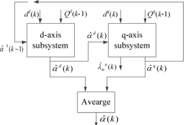
When RTLS is used to estimate the parameters of PMSM directly, the measured vector d(k) becomes a matrix according to the PMSM model (1). Then the recursive matrix Q(k) needs to calculate the matrix inversion at each recursion, which results in heavy computational burden and should usually be avoided for online algorithm. A coupled RTLS (CRTLS) is proposed to reduce computation load for each iteration. The coupled identification is an effective method for multi-input multi-output (MIMO) system [17].
The schematic diagram of the CRTLS for PMSM is
) ( ˆd k a aˆq(k) ) 1 ( ˆqk -a ) ( ˆq k m l ) ( ˆ k a ) ( ˆd k a
shown in Fig. 3. The variables denote a vector or matrix in
d-axis subsystem for superscript “d ” or q-axis subsystem
for superscript “q”. The PMSM model is decomposed into two subsystems (d-axis subsystem and q-axis subsystem). Each subsystem is estimated by RTLS. The common parameters for dq axis subsystems are Rs, Ld and Lq. Define the common parameter vector
)] ( ) ( ) ( [ ) (k = Rs k Ld k Lq k
a
For k-th estimation cycle, d-axis subsystem replaces ˆd
a (k-1) with ˆq
a (k-1), and q-axis subsystem replaces ˆq
a (k-1) with ˆd
a (k). In this way the latest estimated common parameter vector ˆa is always used for the next iteration of another subsystem. Such operations are based on the theory of Jacobi and Gauss-Seidel iterations [17]. Finally, CRTLS sets the average of common parameters estimated by each subsystem as the estimated result, while the rest of estimated parameters keep themselves.
For d-axis subsystem, the model is the first expression in (1) and can be rewritten as the following for k-th iteration:
T s ' ] ][ ) ( ) ( ) ( ) ( [ ) ( d d q d q d k i k i k k i k R L L u = -
w
Based on the model, the measured vector dd(k) and measured data matrix Cd(k) are
' ( ) [ ( ) ( ) ( ) ( ) ( )] d d d q d d k = i k i k -w k i k u k (36) ' ' ' (1) (1) (1) (1) (1) (2) (2) (2) (2) (2) ( ) ( ) ( ) ( ) ( ) ( ) d d q d d d d q d d d q d i i i u i i i u C k i k i k k i k u k é - ù ê ú -ê ú = ê ú ê - ú ë û M M M M w w w (37)
It is clear that matrix Cd(k) is composed of k measured vectors dd(1), dd(2), …, dd(k).
For k-th estimation cycle, RTLS for d-axis subsystem has input data including the measured vector dd(k), recursive matrix Qd(k-1) and the common parameter vector
ˆq
a (k-1), and outputs the new recursive matrix Qd(k) and the estimated common parameter vector ˆd
a (k). Matrix Qd(k) can be updated according to (27). The vector
vm+1d(k-1) in (29) corresponding to ˆaq (k-1) can be calculated as: 1 ˆ [ ( 1) 1] ( 1) ˆ [ ( 1) 1] q d m q k v k k + - -- = - -a a (38)
(38) obtains the vector vm+1d(k-1) by the estimated parameter vector, whose function is opposite to (35) .Then vector vm+1d(k) can be calculated according to (29) and (33). At last, ˆd
a (k) can be obtained according to (35). The procedure of d-axis subsystem for k-th estimation cycle is listed in the following:
RTLS for d-axis subsystem: Input: dd(k), Qd(k-1), ˆaq(k-1) Output: Qd(k), ˆad(k) Ÿ Update Qd (k) from (27) Ÿ Get vm+1d(k-1) from (38) Ÿ Get gd (k) from (29) Ÿ Get vm+1d(k) from (34) Ÿ Get ˆad(k) from (35)
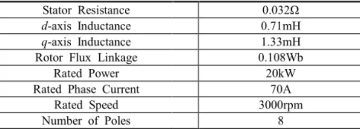
Table 1. Nominal parameters of a prototype PMSM
Stator Resistance 0.032Ω
d-axis Inductance 0.71mH
q-axis Inductance 1.33mH
Rotor Flux Linkage 0.108Wb
Rated Power 20kW
Rated Phase Current 70A
Rated Speed 3000rpm
Number of Poles 8
For q-axis subsystem, the model is the second expression in (1) and can be rewritten as the following for
k-th iteration: ' T s ( ) [ ( ) ( ) ( ) ( ) ( )][ ] q q d q d q m u k = i k w k i k i k w k R L L l
Based on this model, the measured vector dq(k) and measured data matrix Cq(k) are
' ( ) [ ( ) ( ) ( ) ( ) ( ) ( )] q q d q q d k = i k w k i k i k w k u k (39) ' ' ' (1) (1) (1) (1) (1) (1) (2) (2) (2) (2) (2) (2) ( ) (1) ( ) ( ) ( ) ( ) ( ) q d q q q q d q q q d q q i i i u i i i u C k i k i k i k k u k é ù ê ú ê ú = ê ú ê ú ë û M M M M M w w w w w w (40)
The q-axis subsystem has the same process as d-axis subsystem. The vector vm+1q(k-1) in (29) corresponding to
ˆd
a (k) can be calculated as:
1 ˆ ˆ [ ( ) ( 1) 1] ( 1) ˆ ˆ [ ( ) ( 1) 1] d q m m d m k k v k k k + - -- = - -a l a l (41) Matrix Qq(k), vector v
m+1q(k), the estimated common parameter vector ˆq
a (k) and the estimated flux linkage ˆ
m
l (k) also can be calculated as d-axis subsystem does. The procedure of q-axis subsystem for k-th estimation cycle is listed in the following:
RTLS for q-axis subsystem
Input: dq(k), Qq(k-1), ˆad(k), ˆl (k-1) m Output: Qq(k), ˆaq(k), ˆl (k) m Ÿ Update Qq (k) from (27) Ÿ Get vm+1q(k-1) from (41) Ÿ Get gq (k) from (29) Ÿ Get vm+1q(k) from (34) Ÿ Get ˆaq (k) and ˆl (k) from (35) m
For the common parameters in the two subsystems, CRTLS takes their average as the estimations. For the other parameters in the subsystems, CRTLS directly uses the estimations obtained by the subsystems. Then the parameter vector estimated by CRTLS can be expressed as
CRTLS m
ˆ ( )k =[ ( ) ˆ k ˆ ( )]k
q a l (42)
where ˆa (k) is set as following: ˆ( )k =(ˆd( )k + ˆq( )) / 2k
a a a (43)
3.5 Consideration of saturation and cross-coupling effects
The proposed algorithm is based on the assumption that
d-axis and q-axis are independent of each other. But there
exist some effects for the practical PMSM such as magnetic saturation and cross-coupling, which lead to a coupled relation between d-axis and q-axis. To include the influence of the two effects, the d-axis inductance Ld and q-axis inductance Ld in the PMSM model (1) can be modeled as a relation between d-axis and q-axis. To include the influence of the two effects, the d-axis inductance Ld and q-axis inductance Ld in the PMSM model (1) can be modeled as a function of both the dq-axis currents and are denoted by Ld(id, iq) and Lq(id, iq) respectively. And these functions are usually approximated as the exponential function [18] or polynomial expressions [19]. When Ld and Lq in the PMSM model (1) are replaced by the approximation functions, the d-axis and
q-axis could be regarded as a decoupled relationship. The
proposed CRTLS algorithm will be still applicable to the modified model with some changes.
In this paper, the PMSM model (1) is still used because this model is accurate enough for most PMSM applications. The influence of the two effects is in small measure up to the rated current levels because of the large air gap and the magnet’s equivalent air-like gap [20].
4. Simulation and Experimental Results
4.1 Simulation results
The proposed CRTLS algorithm was demonstrated by Matlab/Simulink. A vector control was simulated to generate PMSM running data. The parameters of a prototype PMSM
used in the simulation are listed in Table 1. The simulation was calculated by a fix-step solver with step size 5μs. SVPWM switching frequency and stator current sample period are 5kHz and 200μs respectively.
For comparison, CRTLS, TLS and RLS were applied to estimate the parameters of PMSM with a sudden load torque change. The load torque of PMSM was set to 10N.m at the startup and step to 20N.m after a second at a constant rotor speed 300rpm. Two subsystems of CRTLS algorithm have the following initial values: ˆad(0) = [0 0 0]T, ˆl (0) m
=0, vm+1d(0)= [0 0 0 1]T, vm+1q(0)= [0 0 0 0 1]T, Matrix
Qd(0)= Qq(0)=105I where IÎ R5×5 is an identity matrix. Table 2 shows the parameters estimated by different algorithms at time 2.5s with such load torque. It is clear that the four parameters estimated by CRTLS have less error (maximum error is 3.75%, minimal error is 1.20%) than the ones estimated by RLS. CRTLS performs better due to considering both the errors of input variables and output variables at the same time.
According to Table 2, the parameters estimated by CRTLS are very close to the ones estimated by TLS. This indicates that the approximation of RTLS and coupled implementation of RTLS are feasible for TLS to estimate parameters of PMSM. CRTLS is generally preferred over TLS in view of the computational burden and computer memory.
To confirm the performance with noise interference for the proposed CRTLS algorithm, we injected Gauss noise to
d-axis and q-axis currents respectively. The estimated
processes for CRTLS and RLS are shown in Fig. 4. It can be seen that both the proposed CRTLS and standard RLS can converge to the true values and the former has higher accuracy.
To quantitatively evaluate the enhancement brought by the proposed algorithm, the relative error vector and the mean square deviation (MSD) are defined as follow:
T s s ( ) ( ) ( ) ( ) ( ) ( ) ( ) ( ) q d m k d q m L k R k L k k e R k L k L k k éD D D Dl ù = ê ú l ê ú ë û (44) 2 10 F MSD=10 log ( (´ E ek )) (45)
where Rs(k), Ld( k ), Lq( k ), and λm(k) are the estimated parameters and ΔRs( k ), ΔLd( k ), ΔLq( k ), and Δλm( k ) are the identification absolute error at the k-th estimation cycle. The MSD with the unit of dB is used as the evaluation index. The MSDs for different algorithms are shown in Fig. 4. It is shown that the proposed algorithm Table 2. The estimated results for the simulations
RLS CRTLS TLS
Parameters True Value
Estimated Value Error Estimated Value Error Estimated Value Error
Rs [Ω] 0.032 0.0358 11.87% 0.0332 3.75% 0.0330 3.12%
Ld [mH] 0.71 0.653 -8.03% 0.688 -3.10% 0.689 -2.96%
Lq [mH] 1.33 1.273 -4.29% 1.292 -2.86% 1.293 -2.78%
generates lower MSDs than the standard RLS algorithm. The proposed algorithm yields a MSD reduction of 8.98 dB compared to the RLS algorithm at the end of the
simulation, which suggests an improved accuracy for the estimated parameters.
4.2 Experimental Results
In order to verify the proposed CRTLS algorithm, experiments were carried out. The hardware platform of the DSP-based vector control system is shown in Fig. 5. DSP TMS320F28335 with a clock frequency of 150MHz is used to execute the control algorithm. The inverter switching frequency and sample period are 5kHz and 200us, respectively. The parameters of PMSM are listed in Table 1. This machine was designed for electric vehicle drives. The load is an eddy current retarder.
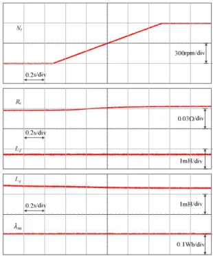
Two operating conditions are adopted to verify the feasibility of the proposed algorithm. Condition 1 has a sudden load torque change from 10N.m to 20N.m at constant rotor speed 300rpm. Condition 2 performs a sudden rotor speed change from 300rpm to 600rpm at constant load torque 10N.m.
Table 3 shows the experimental results for the two conditions. For Condition 1, the estimated stator resistance has the maximum error of -6.87% and rotor flux linkage
Fig. 4. Simulation results under a sudden change in load torque at a constant rotor speed
Fig. 5. Experimental setup of PMSM drive system
Fig. 6. Experimental results under a change in rotor speed at a constant load torque
Table 3. The estimated results for the experiments
Condition 1 Condition 2
Parameters value True Estimated value Error Estimated value Error Rs [Ω] 0.032 0.0298 -6.87% 0.0305 -4.69% Ld [mH] 0.71 0.755 6.34% 0.749 5.49% Lq [mH] 1.33 1.392 4.66% 1.381 3.83% λm [Wb] 0.108 0.1055 -2.31% 0.1061 -1.76%
has the minimum error of -2.31%. Condition 2 has less error than Condition 1 does. The changes of the estimated parameters for Condition 2 are shown in Fig. 6. The estimated stator resistance and q-axis inductance approach to the true values a little during the acceleration. While the estimated d-axis inductance and rotor flux linkage are not affected.
Comparing the experimental results with the simulation results for Condition 1, the former has more error. There are several reasons for this. Firstly, there are some differences between the model of PMSM and the real motor. The effects such as magnetic saturation, motor loss, et al, are not included in the model. Secondly, the measured currents and rotating speed may have measurement error due to noise, electromagnetic interference or the measuring devices. This condition can be ignored for the simulations. Thirdly, the true values of PMSM parameters may vary with operation temperature and stator currents in the practical application.
Another experiment is conducted to further verify the performance of the proposed algorithm on the PMSM with vector control. The operations of id=0 and different iq are performed on the experimental machine. The influence of saturation and cross-couple effects is considered. The dq-axis inductances are measured by an offline method based on the PMSM model (1), which performs the operations at a locked-rotor position. The measured and estimated dq-axis inductances are shown in Fig. 7. It can be seen that d-axis inductance almost keep a constant for different iq. The measured q-axis inductance has little changes when iq is less than 50A, and then becomes less for a bigger iq, which is resulted by the effect of saturation. The results of d-axis inductance estimation have an average error of 5.21%
and a maximum error of 5.70%. The average error and maximum error for the q-axis inductance estimation are 4.65% and 6.08% respectively. It is also observed that the estimated q-axis inductance can follow the variation of the measured q-axis inductance due to saturation.
5. Conclusion
According to the coupled identification and the total least squares identification technique, this paper proposes the online parameter estimation method using the CRTLS algorithm for PMSM. The algorithm can simultaneously estimate stator resistance, rotor flux linkage, d-axis inductance and q-axis inductance. The effectiveness of the proposed algorithm has been demonstrated through the Simulink-based simulation results and the PMSM experi-mental results. The presented algorithm is applicable to interior and surface-mount PMSM.
Acknowledgements
This work was supported in part by the Natural Science Foundation of Zhejiang Province of China (LY16F020025) and in part by the Quality and Supervision Scientific Research Project of Zhejiang Province of China (20180356).
References
[1] J. Kim, I. Jeong, K. Lee, and N. Kwanghee, “Fluctuating current control method for a PMSM along constant torque contours,” IEEE Trans.
Power Electronics, vol. 29, no. 11, pp. 6064-6073,
Nov. 2014.
[2] O. Sandre-Hernandez, R. Morales-Caporal, J. Rangel-Magdaleno, and P. Heregrina-Barreto, “Parameter identification of PMSMs using experimental measurements and a PSO algorithm,” IEEE Trans.
Instrumentation and Measurement, vol. 64, no. 8, pp.
2146-2154, Aug. 2015.
[3] T. L. Vandoorn, F. M. D. Belie, T. J. Vyncke, et al., “Generation of multisinusoidal test signals for the identification of synchronous-machine parameters by using a voltage-source inverter,” IEEE Trans.
Industrial Electronics, vol. 57, no. 1, pp. 430-439, Jan.
2010.
[4] S. J. Underwood and I. Husain, “Online Parameter Estimation and Adaptive Control of Permanent-Magnet Synchronous Machines,” IEEE Trans. Industrial
Electronics, vol. 57, no. 7, pp. 2435-2443, Jul. 2010.
[5] S. Kallio, J. Karttunen, P. Peltoniemi and O. Pyrhonen, “Online Estimation of Double-Star IPM Machine Parameters Using RLS Algorithm,” IEEE Trans. Fig. 7. Experimental results of dq-axis inductance
Industrial Electronics, vol. 61, no. 9, pp. 4519-4530,
Sep. 2014.
[6] H. W. Sim, J. S. Lee and K. B. Lee, “On-line Parameter Estimation of Interior Permanent Magnet Synchronous Motor using an Extended Kalman Filter,”
Journal of Electrical Engineering & Technology,
vol. 9, no. 2, pp. 600-608, 2014.
[7] B. Thierry, L.Nicolas, N.M. Babak and M. T. Farid, “Online identification of PMSM parameters: Parameter identifiability and estimator comparative study,”
IEEE Trans. Industry Applications, vol. 47, no. 4, pp.
1944-1957, Jul. 2011.
[8] K. Liu and Z. Q. Zhu, “Position-Offset-Based Parameter Estimation Using the Adaline NN for Con-dition Monitoring of Permanent-Magnet Synchronous Machines,” IEEE Trans. Industrial Electronics, vol. 62, no. 4, pp. 2372-2383, Apr. 2015.
[9] Z. H. Liu, H. L. Wei, Q. C. Zhong, et al., “Parameter Estimation for VSI-Fed PMSM Based on a Dynamic PSO With Learning Strategies,” IEEE Trans. Power
Electronics, vol. 32, no. 4, pp. 3154-3165, Nov.
2017.
[10] D. Q. Dang, M. S. Rafaq, H. H. Choi and J. W. Jung, “Online Parameter Estimation Technique for Adaptive Control Applications of Interior PM Synchronous Motor Drives,” IEEE Trans. Industrial Electronics, vol. 63, no. 3, pp. 1438-1449, Mar. 2016.
[11] R. Arablouei, K. Dogancay and S. Werner, “Recursive Total Least-Squares Algorithm Based on Inverse Power Method and Dichotomous Coordinate-Descent Iterations,” IEEE Trans. Signal Processing, vol. 63, no. 8, pp. 1941-1949, Aug. 2015.
[12] T. Kim, Y. Wang, Z. Sahinoglu, et al., “A Rayleigh Quotient-Based Recursive Total-Least-Squares Online Maximum Capacity Estimation for Lithium-Ion Batteries,” IEEE Trans. Energy Conversion, vol. 30, no. 3, pp. 842-851, Aug. 2015.
[13] S. Rhode, F. Gauterin, “Online Estimation of Vehicle Driving Resistance Parameters with Recursive Least Squares and Recursive Total Least Squares,” in IEEE
Intelligent Vehicles Symposium, Gold Coast, Australia,
June 2013.
[14] M. Brand, “Incremental singular value decomposition of uncertain data with missing values,” in
Pro-ceedings of ECCV2001 Conference, Copenhagen,
Denmark, May 2002.
[15] H. Wu, S. X. Chen, H. Y. Zhang, et al., “Robust recursive total least squares passive location algorithm,” Journal of Central South University (Science and Technology), vol. 46, no. 3, pp. 886-893, Mar. 2015.
[16] T. Söderström, “Errors-in-variables methods in system identification,” Automatica, vol. 43, no. 6, pp. 939-958, Jun. 2007.
[17] Z. W. Shi, Y. Wang, and Z. C. Ji, “Bias compensation based partially coupled recursive least squares
identification algorithm with forgetting factors for MIMO systems: Application to PMSMs,” Journal of
the Franklin Institute, vol. 353, no. 13, pp.
3057-3077, Mar. 2016.
[18] B. Stumberger, G. Stumberger, D. Dolinar, et al., “Evaluation of Saturation and Cross-Magnetization Effects in Interior Permanent-Magnet,” IEEE Trans.
Industry Applications, vol. 39, no. 5, pp. 1264-1271,
Sep. 2003.
[19] A. Rabiei, T.Thiringer, M. Alatalo, et al., “Improved Maximum-Torque-Per-Ampere Algorithm Account-ing for Core Saturation, Cross-CouplAccount-ing Effect, and Temperature for a PMSM Intended for Vehicular Applications,” IEEE Trans. Transportation
Electri-fication, vol. 2, no. 2, pp. 150-159, Jun. 2016.
[20] R. Krishnan, Permanent Magnet Synchronous and
Brushless DC Motor Drives: CRC, 2010, pp.
226-231.
Yangding Wang He received the M.S. degree in Mechatronics Engineering from Hangzhou Dianzi University, China, in 2008. Since 2009, he has been a senior engineer with the Ningbo Academy of Product Quality Supervi-sion & Inspection. His research intere-sts include measurement, testing and standardization.
Shen Xu He received his B.S., M.S. and Ph.D. degrees in Electronic Engineering from Southeast University, China, in 2001, 2003 and 2008 respec-tively. Since 2009, He has been a lecturer with the School of Information and Technology, Zhejiang Sci-Tech University, China. He is a currently also a Postdoctoral Fellow with the College of Electrical Engineering, Zhejiang University, China. His research interests include motor drives and parameter estimation.
Hai Huang He received the M.S. degree in Computer Science from Xihua University, China, in 2006, and the Ph.D. degree in Computer Science from Shanghai Jiaotong University, China, in 2010. Since 2012, he has been an Associate Professor with the School of Information and Technology, Zhejiang Sci-Tech University, China. His research interests include security and motor drives.
Yiping Guo She received the B.S. degree in Material Science from Zhejiang University, China, in 1984. Since 2015, she has been a senior engineer with a rank of professor with the Ningbo Academy of Product Quality Supervision & Inspection. Her research interests include measurement, testing and standardization.
Hai Jin He received the M.S. degree in Electrical Engineering from HeFei University of Technology, China, in 2002, and the Ph.D. degree in Electrical Engineering from Zhejiang University, China, in 2006. Since 2008, he has been an Associate Professor with the School of Information and Technology, Zhejiang Sci-Tech University, China. His research interests include motor drives and parameter estimation.
![Fig. 2. The difference between LS and TLS ˆ ( ) 0 1C+ DCæç ö÷ = -è øq (18) where C = [ H y ] and D C = [ F e ]](https://thumb-ap.123doks.com/thumbv2/123dokinfo/4889696.36714/3.892.520.754.142.464/fig-difference-ls-tls-ˆ-c-dcæç-øq.webp)