Full Terms & Conditions of access and use can be found at
https://www.tandfonline.com/action/journalInformation?journalCode=tabe20
Journal of Asian Architecture and Building Engineering
ISSN: 1346-7581 (Print) 1347-2852 (Online) Journal homepage: https://www.tandfonline.com/loi/tabe20
Spatial and Temporal Effects of Built Environment
on Urban Air Temperature in Seoul City, Korea: An
Application of Spatial Regression Models
Sugie Lee, Jaehyun Ha & Hyemin Cho
To cite this article: Sugie Lee, Jaehyun Ha & Hyemin Cho (2017) Spatial and Temporal Effects of Built Environment on Urban Air Temperature in Seoul City, Korea: An Application of Spatial Regression Models, Journal of Asian Architecture and Building Engineering, 16:1, 123-130, DOI: 10.3130/jaabe.16.123
To link to this article: https://doi.org/10.3130/jaabe.16.123
© 2018 Architectural Institute of Japan
Published online: 24 Oct 2018.
Submit your article to this journal
Article views: 45
Spatial and Temporal Effects of Built Environment on Urban Air Temperature
in Seoul City, Korea: An Application of Spatial Regression Models
Sugie Lee*1, Jaehyun Ha2 and Hyemin Cho3
1 Associate Professor, Department of Urban Planning and Engineering, Hanyang University, Korea 2 Ph.D. Student, Department of Urban Planning and Engineering, Hanyang University, Korea 3 Graduate Student, Department of Urban Planning and Engineering, Hanyang University, Korea
Abstract
In this study we examined the relationships between the built environment and urban air temperature in Seoul city, Korea. We developed multivariate regression models that address the relationship between built environment characteristics and the ambient air temperature with spatial statistics techniques. In addition, we analyzed the difference in daytime and nighttime air temperature to identify the built environment characteristics that affect the intensity of the nocturnal urban heat island effect (UHI). The large sample size of AWS locations in Seoul makes it possible to analyze the factors that influence ambient air temperature and UHI effect. The analysis results indicate that the sky view factor (SVF) and gross floor area significantly influence the daytime air temperature, while the building coverage and albedo showed strong relationships with the nocturnal air temperature. This study also demonstrated the importance of advanced spatial statistics techniques that control spatial autocorrelation and spatial heteroscedasticity in urban air temperature research. Our models confirmed the need to capture the effects of spatial autocorrelations within our spatial data. The findings of this study are valuable for understanding the complicated associations between the built environment and urban air temperature and to develop public policies to mitigate UHI effects.
Keywords: air temperature; built environment; urban heat island effect; automatic weather stations; spatial statistics 1. Introduction
During the past several decades, urban planners and public policy makers have had great concerns about the impact of built environments on urban climate. Many studies have already tried to address the relationship between surface temperature and land use or land cover. Other studies focused on air temperature and its determining factors. In particular, urban scholars are interested in the urban heat island effect and its driving forces. Previous studies on the urban heat island effect however, have not fully addressed the impacts of three-dimensional characteristics and spatial autocorrelations in the analysis models (Chun and Guldmann, 2014).
This study examines the relationship between built environment and the urban heat island effect in Seoul city, Korea. We focused on the impact of urban built environmental fabrics on ambient urban temperature. The data source we used is the "SK Automatic Weather Stations (AWS) API", which provides ambient
temperature, humidity, and wind direction and velocity. Apart from the 30 AWS locations managed by the government, this study also employed the 295 AWS across Seoul city, which improved the accuracy of analysis.
We built a dataset for the built environment factors and urban ambient temperature. Then, we developed multivariate regression models that addressed the relationship between the built environment factors and urban heat island effect during daytime and nighttime. From the multivariate regression models, we identified determinant factors of the built environment that have a significant impact on urban heat island effects. Lastly, we suggest urban planning and design policies that could mitigate urban heat island effects in the city of Seoul.
2. Literature Review
Climate change and the urban heat island (UHI) effect have been increasingly important issues in urban and regional planning. Urban heat island effects indicate that the air temperature of urban areas is relatively higher than that of rural areas. Rapid urbanization has transformed open spaces into built-up areas with buildings, roads, and other impervious surfaces, which may increase surface temperature as well as air temperature. Many studies have already
*Contact Author: Sugie Lee, Associate Professor,
Dept. of Urban Planning & Engineering, Hanyang University, 222 Wangsimniro, Seongdong-gu, Seoul 04763, Korea
Tel: +82-2-2220-0417 Fax: 82-2-2220-1945 E-mail: [email protected]
( Received April 6, 2016 ; accepted December 1, 2016 )
124 JAABE vol.16 no.1 January 2017 Sugie Lee
addressed the relationship between land surface temperature (LST) and urbanization (Oke, 1976; Jenerette et al., 2007; Yuan and Bauer, 2007; Xiao et
al., 2007).
Scholars have also tried to address the relationship between land use/land cover and air temperature (Bowler et al., 2010; Shudo et al., 1997; Jusuf et
al., 2007). Bowler et al. (2010) asserted that green
space can moderate the air temperature in urban environments. In addition, Shashuabar and Hoffman (2000) argued that many small-scale distributed green spaces would be beneficial for reducing air temperature. Trees provide substantial benefits for pedestrians by shading street canyons during the hot summer and also have a cooling effect on air temperature. Jusuf et al. (2007) pointed out that we could improve the urban environment through land use planning because land use/land cover has a significant impact on urban temperature.
The UHI effect is the outcome of complicated interactions among many determinant factors. Beyond basic determinant factors such as humidity, wind speed, and altitude, UHI is strongly associated with human activities including urban development that change land use and land cover (Jusuf et al., 2007; Schwarz et al., 2012). In addition, three-dimensional urban environment factors (along with urban canyon effects) may have significant impacts on air temperature and UHI effects because they affect air circulation, wind flow, area shaded by buildings, and so on. Higher floor area ratios and higher building footprint areas reduce the speed of wind (Kubota et
al., 2008). In addition, urban design measures such
as sky view factors, obtained from the relationship between height and spacing of buildings, have an important effect on urban temperature (Barring et
al., 1985; Giridharan et al., 2004). Gál et al. (2009)
reported a strong linear negative association between annual mean temperatures and SVF. Other studies also showed statistically significant associations between SVF and urban temperature (Chen et al., 2012; Unger, 2009; Svensson, 2004).
Chun and Guldmann (2014) pointed out the shortcomings in previous UHI studies noting that 2-D information rather than 3-D information was used, a small set of variables was used and a simple ordinary least squares was used that cannot control spatial autocorrelation. They examined the association between three-dimensional urban design factors and LST using a spatial statistics technique that can control for spatial autocorrelation. Their study included solar radiation, sky view factor, building floor area ratios by type, building volume, roof-top areas, ratio of building height to road width, open space, and vegetation for the city of Columbus, Ohio. They concluded that solar radiation, open spaces, vegetation, building roof-top areas, and water have strong impacts on surface temperatures using spatial statistics that capture
neighboring effects. Similarly, Giridharan et al. (2004) examined design-related variables on the outdoor micro-level daytime heat island effect in a residential development in Hong Kong. They concluded that energy efficient design can improve the urban thermal environment by manipulating surface albedo, sky view factor, and total height to floor area ratio.
Although previous studies over the past several decades have tried to address the UHI effect and its determinant factors, they have a few critical limitations. First, most studies have focused on land surface temperature because the land coverage data and land surface temperature information are available from satellite imagery. However, the UHI effect should be addressed with air temperature measurements. A couple of studies used air temperature obtained from automatic weather station (AWS) information, but these studies are usually limited due to small sample sizes. Second, most existing studies have focused on two-dimensional land coverage information to examine its impact on land surface temperature. However, two-dimensional land coverage information may have a limited impact on air temperature. Actually, air temperature may have significant correlations with three-dimensional urban environments such as building height, building spacing, sky view factor, and open space in addition to meteorological effects like humidity, wind speed, and altitude. Third, methodological advances in statistical analysis should be applied for analyzing the UHI and its determinant factors. Most existing studies have employed simple OLS regression models. However, as a recent study of Chun and Guldmann (2014) indicated, research on LST or UHI should employ advanced statistical methods that control for spatial autocorrelation and spatial heterogeneity.
3. Case Study and Methodology 3.1 Case Study Area
This study focuses on Seoul, the capital city of Korea. Seoul is one of the most populated cities in the world with an area of 605km2 and a population
density of 17,000 people/km2 (Demographia
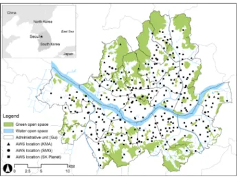
World Urban Areas, 2016). Seoul accommodates more than 10 million people and has a variety of geographical characteristics with mountainous terrain, a river and streams (see Fig.1.). In addition, built environments in Seoul are very diverse, including high-density residential complexes, middle-and low-density residential areas, and commercial and industrial districts. Due to global climate change and the increasing air temperature in Seoul, demands for managing the urban thermal environment are increasing. For example, the highest air temperature recorded last year (2015) was 36.0°C on 11 July, and there were two heat wave warnings, which are issued when the hottest daily temperature exceeds 33.0°C for two days or more.
As seen in Fig.1., 295 AWSs are evenly distributed across the city of Seoul. Compared to most previous studies such as Chen et al. (2012) and Giridharan et al. (2008) that focus on urban air temperature with a small number of AWSs, the level of spatial resolution of AWSs in this study enables us to examine the various attributes of the built environment in modeling urban air temperature during the day and night.
3.2 Dependent Variable
Most of the previous studies that analyzed the urban temperature have focused on the land surface temperature (LST) extracted from the satellite images. Therefore, the analysis results of previous LST studies have critical limitations because there are differences between LST and the air temperature. By using the air temperature information observed from the AWSs, we were able to analyze realistic effects of built environments on air temperature.
The dependent variable is air temperature, observed by 295 AWSs in Seoul. The locations of the AWSs is
shown in Fig.1. Among these 295 AWSs, 240 AWSs are managed by the 'SK Planet' company, and the others are operated by government organizations including the Korea Meteorological Administration (KMA) and the Seoul Metropolitan Government (SMG). All of the AWS were authenticated as having standard equipment. However, the 11 AWS sites operated by the Korea Meteorological Administration were incapable of observing humidity, and were therefore finally excluded from our analysis data. Even so, our analysis results covered the entire city of Seoul since the remainder of the sites were widely distributed as shown in Fig.1.
We collected climate information such as air temperature, humidity, and wind strength observed on 11 July, 2015, since it was reported as the hottest day in 2015. Moreover, since our research focused on the temporal effect of UHI, we used the average air temperature observed during both day and night. We have selected our study periods as 10AM-6PM, and 9PM-11PM for day and night, respectively. In the case of the daytime, we identified the time period when the air temperature was above 30ºC. On the other hand, 9PM-11PM was selected as the nighttime based on the work of Oke (1981), who argued that the nocturnal UHI occurs 3-5 hours after sunset.
3.3 Independent Variables
As presented in Table 1., selected variables include the properties of AWS, climate characteristics, and two and three-dimensional urban environment indices. The detailed descriptions of each variable are as follows:
First, the elevation of each AWS location was used since the air temperature was expected to be different based on the altitude. Second, climate characteristics such as the wind velocity and humidity were used as the control variables. Those variables, measured by
Table 1. Description of Variables
Category Variables Definition Unit Data source*
AWS
AWS elevation Altitude of each AWS m KMA / SMG /
SK Planet (11 July, 2015) Air temperature Average air temperature of day and night time ºC
Wind velocity Average wind velocity of day and night time m/s
Humidity Average humidity of day and night time %
Built Environ-ment
Building coverage Proportion of built area (area of the building footprint / area of urban zone) % New Address Database, 2015 Green area ratio Proportion of green area(area of green / area of the 500m circular buffer) % Biotope Map Database, 2014 Albedo Albedo index calculated using satellite image(using the DN value of Landsat 8 image) - Landsat 8 image(30, May, 2014) Surface solar radiation Amount of surface solar radiation for all day MJ/ m2 ArcMap Solar
Radiation Tool Proximity to natural open
space Minimum length between natural open space and the AWS location point m New Address Database, 2015 Road width Average road width for each 500m circular buffer m
Sky view factor (SVF) Areal SVF calculated for each buffer using the 'Skyline Graph' tool in ArcScene - New Address Database, 2015 Building Ledger Database, 2015 GFA_res (residential use) Gross floor area of residential use inside the 500m circular buffer m2
GFA_com (commercial use) Gross floor area of commercial use inside the 500m circular buffer m2
* Korea Meteorological Administration (KMA); Seoul Metropolitan Government (SMG) Fig.1. Locations of AWS in Seoul City
126 JAABE vol.16 no.1 January 2017 Sugie Lee
each AWS, were provided with the air temperature data by each organization operating AWS equipment in Seoul. We have selected those variables because wind velocity and humidity significantly affect the air temperature. Third, two-dimensional urban environment indices such as the surface albedo, surface solar radiation, road width, and green area, and the proximity to natural open spaces were used as the independent variables. Those variables were calculated based on the 500m circular buffer drawn for each AWS location point in ArcGIS software. For the road width, we selected this variable because it may affect both the ventilation and solar radiation. Therefore, we assume that the average road width is more likely to be associated with urban air temperature. We calculated the average road width within the 500m circular buffer. The surface albedo was computed using the equation developed in previous studies using the Landsat 8 satellite image. Surface solar radiation was calculated using the 3D dataset of Seoul and the solar radiation tool in ArcMap. Variables such as road and park area, and the proximity value to natural open spaces were calculated using the 2015 New Address database for Seoul.
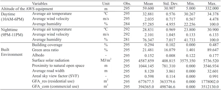
Lastly, three-dimensional indices including the gross floor area of each land use and the sky view factor (SVF) were used. Those urban indices were calculated by using the ArcGIS and the 3D dataset built by linking the 2015 New Address database and building ledger database of Seoul. The descriptive statistics of the variables used in our study are presented in Table 2. Before conducting the analysis, a log transformation was used on the altitude of AWS, albedo, and the gross floor area of residential and commercial uses to adjust them to a normal distribution.
3.4 Methodology
We used multivariate regression models to examine the relationship between the built environment and air temperature. We also included descriptive analysis and advanced spatial statistics. In order to analyze the impact of independent variables on air temperature, we
first applied the OLS regression model. However, the outputs of OLS regression could be biased if spatial autocorrelation and spatial heterogeneity are present. Chun and Guldmann (2014) pointed out that spatial regression models are more suitable (especially when modelling the UHI intensity or the air temperature) because the temperature is predicted to be spatially correlated with the temperature observed nearby.
Therefore, we applied spatial statistics techniques such as Moran's I and spatial statistical models. For the application of spatial statistics, we used 'GeoDa' and 'GeoDaSpace', which are well-known software packages for spatial analysis and modelling developed by the Spatial Analysis Laboratory at Arizona State University (Anselin, 2004; Anselin and Rey, 2014).
To determine the analysis model for our spatial data, the Moran I test and the Breusch Pagan (BP) test were performed. These tests are used to identify the spatial autocorrelation effect and the heterogeneity of the spatial data. We first performed the OLS model using GeoDa software in order to examine the Moran I test result. Then, based on the Moran I test value, we decided whether there was a need to construct a spatial regression model. The spatial regression model has advantages over the simple OLS model, therefore we identified the Lagrange Multiplier (LM test) value of both the spatial lag model and the spatial error model. According to Anselin (2004), the model which shows the higher value in the LM test is more appropriate. Based on the previous decision, we then used the most suitable spatial regression model to analyze the relationships between the independent and dependent variables. Furthermore, by examining the BP test of the selected model, we confirmed whether there is heterogeneity in the estimated residuals.
When we had both spatial autocorrelation and spatial heterogeneity in the OLS model, we conducted a spatial regression model with the KP HET (Kelejian-Prucha consistent estimator for heteroskedastic error terms) option in the GeoDaSpace software. Using the KP HET option, we controlled both the spatial
Table 2. Descriptive Statistics of Variables
Variables Unit Obs. Mean Std. Dev. Min. Max.
Altitude of the AWS equipment m 295 59.600 30.907 5.000 332.000
Daytime Average air temperature ºC 295 32.881 0.576 30.267 34.378
(10AM-6PM) Average wind velocity m/s 295 2.035 0.717 0.567 4.478
Average humidity % 284 57.285 4.955 22.256 100.0
Nighttime Average air temperature ºC 292 28.831 0.969 23.800 30.900
(9PM-11PM) Average wind velocity m/s 292 2.101 1.045 0.133 6.133
Average humidity % 281 76.347 7.017 41.733 100.0
Built Environment
Building coverage % 295 0.294 0.102 0.000 0.487
Green area ratio % 295 21.481 16.079 1.401 89.647
Albedo - 295 0.152 0.008 0.122 0.177
Surface solar radiation MJ/m2
295 4587.859 408.815 3575.350 5736.520 Proximity to natural open space m 295 1044.145 781.310 0.000 3546.934
Average road width m 295 8.120 3.861 0.000 32.601
Areal sky view factor (SVF) - 295 0.598 0.114 0.000 0.991
GFA_res (residential use) m2
295 677677.5 363379.6 0.000 1778002.0 GFA_com (commercial use) m2
autocorrelation effect and the heterogeneity in the regression model (Anselin and Rey, 2014). However, since the indicators of the goodness of fit of the models were not sufficiently provided by the GeoDaSpace software, we only examined whether the analysis results of the spatial regression model without the KP HET option were robust.
4. Analysis and Findings
We discuss our analysis of the association between urban design factors and air temperature in this section. SLM or SEM are useful spatial statistics methods that address the spatial autocorrelation problem. We identified the final model based on the goodness of fit for each spatial regression model. The log-likelihood ratio (LR test), Akaike information criterion (AIC), and Schwarz criterion (SC) were used as the indicators for the goodness of fit. High LR-test values and low AIC and SC values indicated a well-estimated model (Anselin, 2005). In addition, when the heteroscedasticity was a significant problem in the analysis data, we applied SEM with the KP HET option to control the heteroscedasticity (Anselin, 2014).
4.1 Daytime Air Temperature
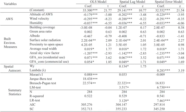
Table 3. shows the analysis results of the association between urban design factors and the daytime air temperature. Moran's I value of the OLS model indicates that the spatial autocorrelation was significant, implying that spatial regression methods were more appropriate in estimating the daytime air temperature.
SLM and SEM were both conducted to capture the effect of spatial autocorrelation. Based on the model decision process described in the prior section, we concluded that SEM showed the best estimated results. As compared to the OLS model, the LR test value increased while the AIC and SC values decreased when SEM was used. Furthermore, the BP test results of the SEM were not statistically significant, implying the absence of heteroscedasticity. Moran's I value of the SEM model implies that the spatial autocorrelation was fully controlled by applying spatial statistics.
Moving on to the estimation results (mainly focusing on the results of SEM), the variables measured from the AWS showed a significant relationship with the daytime air temperature. Specifically, altitude of the AWS, wind velocity, and humidity affected the daytime air temperature negatively. This observation is in agreement with the previous studies. Meanwhile, solar radiation showed a positive relationship with daytime air temperature, which is reasonable.
The average road width showed positive associations, being statistically significant at the 90% confidence level. This result implies that increasing the average road width leads to an increase in daytime air temperature. The coefficient of SVF was negative and significant at the 99% confidence level. Although Giridharan et al. (2007) have stated that an increase in SVF should lead to an increase of air temperature, the results of our study are similar to the conclusion of Chen et al. (2012). They argued that SVF can have both positive and negative effects on daytime air temperature. On the other hand,
Table 3. Estimation Results on Day-time Air Temperature
Variables Coef.OLS Modelt Coef.Spatial Lag Modelz Spatial Error ModelCoef. z
(Constant) 33.300*** 21.77 29.141*** 10.77 32.552*** 21.54 AWS Altitude of AWS -0.179*** -3.00 -0.202*** -3.48 -0.229*** -3.95 Wind velocity -0.295*** -8.23 -0.288*** -8.22 -0.291*** -8.35 Humidity -0.037*** -6.55 -0.036*** -6.55 -0.033*** -6.06 Built Environ. Measures
Building coverage -3.0E-08 -0.04 1.2E-07 0.17 2.8E-07 0.38
Green area ratio 0.002 0.63 0.002 0.63 0.002 0.63
Albedo -0.467 -0.79 -0.408 -0.71 -0.833 -1.41
Surface solar radiation 2.2E-04** 2.09 2.1E-04** 2.01 2.4E-04** 2.27 Proximity to open space 4.2E-05 1.21 3.5E-05 1.05 3.8E-05 0.98
Average road width 0.019* 1.77 0.018* 1.72 0.018* 1.71
Areal sky view factor -1.207*** -2.93 -1.142*** -2.83 -1.235*** -3.04 GFA_res (residential use) 0.071*** 3.62 0.067*** 3.52 0.071*** 3.68 GFA_com (commercial use) 0.054* 1.85 0.049* 1.71 0.049* 1.69 Spatial Autocorr. WyLambda (λ) 0.134* 1.75 0.283*** 3.19 Summary Statistics Moran's I 0.088*** 0.033 -0.009 Jarque-Bera test 18.438*** Breusch-Pagan test 22.574** 22.323** 16.833 LM-test 3.517* 6.730*** N 284 284 284 R-squared 0.522 0.529 0.541 LR-test 3.129* 7.463*** AIC 305.276 304.147 297.814 SC 352.713 355.233 345.250 *** p<0.01; ** p<0.05; * p<0.10
128 JAABE vol.16 no.1 January 2017 Sugie Lee
the coefficients of the gross floor area of residential (GFA_res) and commercial uses (GFA_com) were both positive and significant at 1% and 10%, respectively. This result indicates that both the gross floor area of residential and commercial uses increases daytime air temperature.
Variables including the building coverage, green area ratio, albedo, and proximity to open space were not statistically significant in our analysis models. Coefficients of albedo, proximity to open space, and building coverage fall in line with the general theory, however they were not significant.
4.2 Nighttime Air Temperature
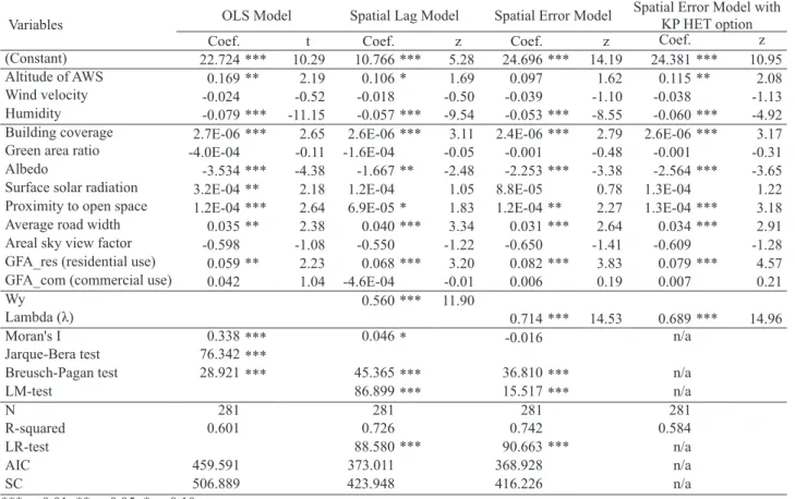
Table 4. presents the analysis results on the relationships between urban design indices and the air temperature at night. As shown in Table 4., while the LR-test value increased, the AIC and SC values decreased dramatically for the SEM model. In other words, the SEM model controlled for spatial autocorrelation which can be indicated through Moran's I value of the SEM model. However, the BP test result of the SEM model was significant, implying the existence of heteroscedasticity. Therefore, we tested the SEM with the KP HET option of GeoDaSpace. However, the indicators of the goodness of fit were not available for the SEM with the KP HET option. In addition, the results did not show great difference from the SEM model. Hence, we focused on the analysis results of the SLM method that were robust.
Among the variables measured by the AWS, only the coefficients of humidity showed a statistical
significance. Wind velocity and the altitude of AWS were not significant for the air temperature at night, which is a different result compared to the result of air temperature in the daytime. Meanwhile, the coefficient of the building coverage was positive and significant at the 99% confidence level. This indicates that an increase in building coverage leads to an increase in air temperature at night. This result also differs from the results of daytime air temperature.
Albedo showed a negative coefficient with nighttime air temperature, indicating that higher albedo decreases nocturnal air temperature. Moreover, the coefficient of proximity to open space was positive. This implies that the increase in distance to open space results in an increase in nighttime air temperature. The coefficients of the road width were positively associated with the nighttime air temperature, while being significant at the 99% confidence level. For the gross floor area of land use, the coefficient of the residential uses was positive and significant, while commercial uses did not show significance. Other independent variables including green area ratio, surface solar radiation, and SVF were not statistically significant in our models. However, the altitude of AWS and the surface solar radiation showed a statistical significance in the OLS model. This finding indicates that the analysis results may vary according to the estimation methods. In other words, if we do not consider the spatial autocorrelation or the heteroscedasticity, we are more likely to have biased results in the statistical analyses.
Table 4. Estimation Results of Nighttime Air Temperature
Variables OLS Model Spatial Lag Model Spatial Error Model Spatial Error Model with KP HET option
Coef. t Coef. z Coef. z Coef. z
(Constant) 22.724 *** 10.29 10.766 *** 5.28 24.696 *** 14.19 24.381 *** 10.95
Altitude of AWS 0.169 ** 2.19 0.106 * 1.69 0.097 1.62 0.115 ** 2.08
Wind velocity -0.024 -0.52 -0.018 -0.50 -0.039 -1.10 -0.038 -1.13
Humidity -0.079 *** -11.15 -0.057 *** -9.54 -0.053 *** -8.55 -0.060 *** -4.92 Building coverage 2.7E-06 *** 2.65 2.6E-06 *** 3.11 2.4E-06 *** 2.79 2.6E-06 *** 3.17 Green area ratio -4.0E-04 -0.11 -1.6E-04 -0.05 -0.001 -0.48 -0.001 -0.31 Albedo -3.534 *** -4.38 -1.667 ** -2.48 -2.253 *** -3.38 -2.564 *** -3.65 Surface solar radiation 3.2E-04 ** 2.18 1.2E-04 1.05 8.8E-05 0.78 1.3E-04 1.22 Proximity to open space 1.2E-04 *** 2.64 6.9E-05 * 1.83 1.2E-04 ** 2.27 1.3E-04 *** 3.18 Average road width 0.035 ** 2.38 0.040 *** 3.34 0.031 *** 2.64 0.034 *** 2.91 Areal sky view factor -0.598 -1.08 -0.550 -1.22 -0.650 -1.41 -0.609 -1.28 GFA_res (residential use) 0.059 ** 2.23 0.068 *** 3.20 0.082 *** 3.83 0.079 *** 4.57 GFA_com (commercial use) 0.042 1.04 -4.6E-04 -0.01 0.006 0.19 0.007 0.21
Wy 0.560 *** 11.90
Lambda (λ) 0.714 *** 14.53 0.689 *** 14.96
Moran's I 0.338 *** 0.046 * -0.016 n/a
Jarque-Bera test 76.342 ***
Breusch-Pagan test 28.921 *** 45.365 *** 36.810 *** n/a
LM-test 86.899 *** 15.517 *** n/a N 281 281 281 281 R-squared 0.601 0.726 0.742 0.584 LR-test 88.580 *** 90.663 *** n/a AIC 459.591 373.011 368.928 n/a SC 506.889 423.948 416.226 n/a *** p<0.01; ** p<0.05; * p<0.10
Putting the analysis results discussed in Section 4.1 and 4.2 together, we can summarize key findings as follows. First, it is necessary to apply spatial regression methods for an analysis of air temperature in daytime or nighttime. Furthermore, appropriate models may vary according to the spatial or temporal characteristics. Second, variables including humidity, average road width, and gross floor area of residential uses (GFA_res) have strong effects on air temperature during the day and nighttime. Other variables showed different results between daytime and nighttime. In particular, solar radiation, SVF and gross floor area of commercial uses were highly related with daytime air temperature, while building coverage was only associated with the nighttime air temperature.
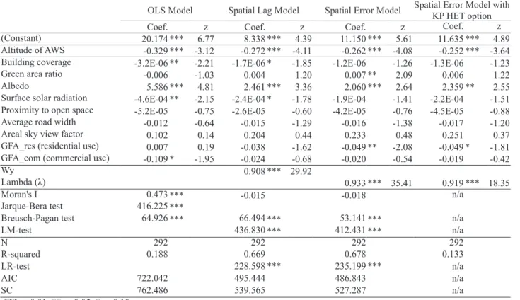
4.3 Differences in Air Temperature between Daytime and Nighttime
The difference in air temperature between daytime and nighttime may be used to identify UHI effects. If high air temperature during the daytime remains at night, we can suspect UHI effects. In this section, we analyzed the association between urban design factors and the air temperature difference between day and night. Analysis results are in Table 5. Low air temperature differences indicate the high intensity of nocturnal UHI because high air temperature differences imply the decrease of air temperature at night. As described earlier, we went through the decision process of the estimation method focusing on the spatial autocorrelation and heteroscedasticity effect of our data. As shown in Table 5., the analysis results of the SEM showed the highest goodness of fit. Furthermore,
the Moran's I value of the SEM shows that the spatial autocorrelation was fully controlled. Meanwhile, since the Breusch-Pagan test result for SEM indicated the existence of heteroscedasticity, we applied the SEM estimation with the KP HET option in GeoDaSpace.
Focusing on the analysis results using SEM, the coefficient of the altitude of AWS was negative and significant. This finding indicates that an increase in the AWS altitude led to a decrease in the air temperature difference between day and night. In the case of the green area ratio and albedo, the coefficients were positive and significant at the 95% confidence level. This result implies that the increase in green area ratio and albedo led to an increase in air temperature difference between day and night. This result further implies that green area ratio and albedo has an effect in mitigating the nocturnal UHI phenomena.
5. Conclusion
In this study, we developed multivariate regression models that address the relationships between urban design factors and the air temperature during the day and night. In addition, by setting the dependent variable as the air temperature difference between day and night, we identified the urban design measures that effect nocturnal UHI intensity. Moreover, we applied spatial statistics techniques to control for the effects of spatial autocorrelation and heteroscedasticity.
The findings of our study indicate that sky view factor (SVF) and the gross floor area have a significant influence on the daytime air temperature, while the building coverage and albedo showed strong correlations
Table 5. Estimation Results on Air Temperature Difference between Day and Night
OLS Model Spatial Lag Model Spatial Error Model Spatial Error Model with KP HET option
Coef. z Coef. z Coef. z Coef. z
(Constant) 20.174 *** 6.77 8.338 *** 4.39 11.150 *** 5.61 11.635 *** 4.89 Altitude of AWS -0.329 *** -3.12 -0.272 *** -4.11 -0.262 *** -4.08 -0.252 *** -3.64 Building coverage -3.2E-06 ** -2.21 -1.7E-06 * -1.85 -1.2E-06 -1.26 -1.3E-06 -1.23
Green area ratio -0.006 -1.03 0.004 1.20 0.007 ** 2.09 0.006 1.22
Albedo 5.586 *** 4.81 2.461 *** 3.36 2.060 *** 2.64 2.359 ** 2.55
Surface solar radiation -4.6E-04 ** -2.15 -2.4E-04 * -1.78 -1.9E-04 -1.41 -2.2E-04 -1.51 Proximity to open space -5.2E-05 -0.75 -2.6E-05 -0.60 -4.2E-05 -0.76 -4.5E-05 -0.88
Average road width -0.012 -0.64 -0.015 -1.29 -0.016 -1.38 -0.017 -1.20
Areal sky view factor 0.102 0.14 0.204 0.44 0.233 0.48 0.251 0.37
GFA_res (residential use) 0.007 0.19 -0.038 -1.62 -0.049 ** -2.08 -0.049 * -1.81 GFA_com (commercial use) -0.109 * -1.95 -0.024 -0.68 -0.020 -0.54 -0.019 -0.42
Wy 0.908 *** 29.92
Lambda (λ) 0.933 *** 35.41 0.919 *** 18.35
Moran's I 0.473 *** -0.015 -0.018 n/a
Jarque-Bera test 416.225 ***
Breusch-Pagan test 64.926 *** 66.494 *** 53.141 *** n/a
LM-test 436.830 *** 412.431 *** n/a N 292 292 292 292 R-squared 0.188 0.669 0.678 0.133 LR-test 228.598 *** 235.199 *** n/a AIC 722.042 495.444 486.843 n/a SC 762.486 539.565 527.287 n/a *** p<0.01; ** p<0.05; * p<0.10
130 JAABE vol.16 no.1 January 2017 Sugie Lee
to the nocturnal air temperature. Moreover, the average road width and the gross floor area of residential uses (GFA_res) were significant variables for both day and night air temperature. Proximity to open space, albedo, and gross floor area of residential uses showed strong correlations to the nocturnal air temperature.
Overall, our study indicated that spatial and temporal issues are very important in determining air temperature due to spatial autocorrelation and heterogeneity. Our models confirmed the importance of capturing the effects of spatial autocorrelation and heteroscedasticity to reach a robust estimation result. We further found that the analysis results using the air temperature measured by AWSs in Seoul slightly differed from the analysis results using the surface temperature extracted by satellite images.
Our results with air temperatures from many AWS sites in Seoul provide a valuable example for how urban air temperature studies can be conducted. Our study also contributes to the literature on estimating the UHI intensity by using the measured air temperature and advanced statistical techniques. However, our study results cannot be generalized because we only focused on the city of Seoul. Moreover, our study results were not able to deal with various built environment measures such as heat sinks or the specific forms of buildings. Thus, additional research should address the relationships between air temperature and urban design factors in large cities using various environmental indices. Furthermore, we suggest research examining the seasonal effect in the relationship between urban indices and air temperature.
Acknowledgements
This work is supported by the Korea Agency for Infrastructure Technology Advancement (KAIA) grant funded by the Ministry of Land, Infrastructure and Transport (Grant 16AUDP-B102406-02). An earlier version of this research was also presented in the 4th International Conference on Countermeasures to Urban Heat Island, National University of Singapore, Singapore on 30 May 2016.
References
1) Anselin, L. (2004). GeoDa: An Introduction to Spatial Data Analysis. Urbana, 51, 61801.
2) Anselin, L. (2005). Exploring Spatial Data with GeoDa: A Workbook. Champaign: Univ. of Illinois, Urbana-Champaign.
3) Anselin, L., and Rey, S. J. (2014). Modern Spatial Econometrics in Practice: A Guide to GeoDa, GeoDaSpace and PySAL. Chicago, IL: GeoDa Press LLC.
4) Barring, L., Mattsson, J. O., and Lindqvist, S. (1985). Canyon Geometry, Street Temperatures and Urban Heat Island in Malmö, Sweden. Journal of Climatology, 5(4), pp.433-444.
5) Bowler, D. E., Buyung-Ali, L., Knight, T. M., and Pullin, A. S. (2010). Urban Greening to Cool Towns and Cities: A Systematic Review of the Empirical Evidence. Landscape and Urban Planning, 97(3), pp.147-155.
6) Chen, L., Ng, E., An, X., Ren, C., Lee, M., Wang, U., and He, Z. (2012). Sky View Factor Analysis of Street Canyons and its Implications for Daytime Intra‐urban Air Temperature Differentials in High‐rise, High‐density Urban Areas of Hong Kong: A GIS‐ based Simulation Approach. International Journal of Climatology, 32(1), pp.121-136.
7) Chun, B., and Guldmann, J. M. (2014). Spatial Statistical Analysis and Simulation of the Urban Heat Island in High-density Central Cities. Landscape and Urban Planning, 125, pp.76-88.
8) Demographia World Urban Areas. (2016). 11th Annual Edition ed. St. Louis: Demographia. Available online: http://www. demographia.com/db-worldua.pdf/ (accessed on 12 October 2016). 9) Gál, T., Lindberg, F., and Unger, J. (2009). Computing Continuous
Sky View Factors using 3D Urban Raster and Vector Databases: Comparison and Application to Urban Climate. Theoretical and Applied Climatology, 95, pp.111-123.
10) Giridharan, R., Ganesan, S., and Lau, S. S. Y. (2004). Daytime Urban Heat Island Effect in High-rise and High-density Residential Developments in Hong Kong. Energy and Buildings, 36(6), pp.525-534.
11) Giridharan, R., Lau, S. S. Y., Ganesan, S., and Givoni, B. (2007). Urban Design Factors Influencing Heat Island Intensity in High-rise High-density Environments of Hong Kong. Building and Environment, 42(10), pp.3669-3684.
12) Giridharan, R., Lau, S. S. Y., Ganesan, S., and Givoni, B. (2008). Lowering the Outdoor Temperature in High-rise High-density Residential Developments of Coastal Hong Kong: The Vegetation Influence. Building and Environment, 43(10), pp.1583-1595. 13) Jenerette, G. D., Harlan, S. L., Brazel, A., Jones, N., Larsen, L.,
and Stefanov, W. L. (2007). Regional Relationships between Surface Temperature, Vegetation, and Human Settlement in a Rapidly Urbanizing Ecosystem. Landscape Ecology, 22(3), pp.353-365.
14) Jusuf, S. K., Wong, N. H., Hagen, E., Anggoro, R., and Hong, Y. (2007). The Influence of Land Use on the Urban Heat Island in Singapore. Habitat International, 31(2), pp.232-242.
15) Kubota, T., Miura, M., Tominaga, Y., and Mochida, A. (2008). Wind Tunnel Tests on the Relationship between Building Density and Pedestrian-level Wind Velocity: Development of Guidelines for Realizing Acceptable Wind Environment in Residential Neighborhoods. Building and Environment, 43(10), pp.1699-1708. 16) Oke, T. R. (1973). City Size and the Urban Heat Island.
Atmospheric Environment, 7(8), pp.769-779.
17) Oke, T. R. (1981). Canyon Geometry and the Nocturnal Urban Heat Island: Comparison of Scale Model and Field Observations. Journal of Climatology, 1(3), pp.237-254.
18) Schwarz, N., Schlink, U., Franck, U., and Großmann, K. (2012). Relationship of Land Surface and Air Temperatures and its Implications for Quantifying Urban Heat Island Indicators— An Application for the City of Leipzig (Germany). Ecological Indicators, 18, pp.693-704.
19) Shashua-Bar, L., and Hoffman, M. E. (2000). Vegetation as a Climatic Component in the Design of an Urban Street: An Empirical Model for Predicting the Cooling Effect of Urban Green Areas with Trees. Energy and Buildings, 31(3), pp.221-235. 20) Shudo, H., Sugiyama, J., Yokoo, N., and Oka, T. (1997). A Study
on Temperature Distribution Influenced by Various Land Uses. Energy and Buildings, 26(2), pp.199-205.
21) Svensson, M. K. (2004). Sky View Factor Analysis–Implications for Urban Air Temperature Differences. Meteorological Applications, 11(3), pp.201-211.
22) Unger, J., Bottyán, Z., Sümeghy, Z., and Gulyás, Á. (2004). Connection between Urban Heat Island and Surface Parameters: Measurements and Modeling. IDŐJÁRÁS/Quarterly Journal of the Hungarian Meteorological Service, 108, pp.173-194.
23) Unger, J. (2009). Connection between Urban Heat Island and Sky View Factor Approximated by a Software Tool on a 3D Urban Database. International Journal of Environment and Pollution, 36, pp.59-80.
24) Xiao, R. B., Ouyang, Z. Y., Zheng, H., Li, W. F., Schienke, E. W., and Wang, X. K. (2007). Spatial Pattern of Impervious Surfaces and their Impacts on Land Surface Temperature in Beijing, China. Journal of Environmental Sciences, 19(2), pp.250-256.
25) Yuan, F., and Bauer, M. E. (2007). Comparison of Impervious Surface Area and Normalized Difference Vegetation Index as Indicators of Surface Urban Heat Island Effects in Landsat Imagery. Remote Sensing of Environment, 106(3), pp.375-386.