1. INTRODUCTION
Motion control of mobile robots is a typical nonlinear tracking control issue and has been discussed with different control schemes such as PID, GPC, sliding mode, predictive control etc[1]-[3]. Intelligent control techniques, based on neural networks and fuzzy logic, have also been developed for path tracking control of mobile robots[4][5]. While conventional neural networks have good ability of self-learning, they also have some limitations such as slow convergence, the difficulty in reaching the global minima in the parameter space, and sometimes even instability as well. In the case of fuzzy logic, it is a human-imitating logic, but lacks the ability of self-learning and self-tuning. Therefore, in the research area of intelligent control, fuzzy neural networks(FNNs) are devised to overcome these limitations and to combine the advantages of both neural networks and fuzzy logic[6][7]. This provides a strong motivation for using FNNs in the modeling and control of nonlinear systems. And the wavelet fuzzy model(WFM) has the advantage of wavelet transform by constituting the fuzzy basis function(FBF) and the conclusion part to equalize the linear combination of FBF with the linear combination of wavelet functions. The conventional fuzzy model can not give the satisfactory result for the transient signal. On the contrary, in the case of WFM, the accurate fuzzy model can be obtained because the energy compaction by the unconditional basis and the description of a transient signal by wavelet basis functions are distinguished[8]. Therefore, we design a FNN structure based on wavelet, which merges these advantages of neural network, fuzzy model and wavelet. The basic idea of wavelet based fuzzy neural network(WFNN) is to realize the process of fuzzy reasoning of WFM by the structure of a neural network and to make the parameters of fuzzy reasoning be expressed by the connection weights of a neural network. And an approach that uses adaptive learning rates is driven via a Lyapunov stability analysis to guarantee the fast convergence. In this paper, we design the direct adaptive control system using the WFNN structure. Through computer simulations, we demonstrate the effectiveness and feasibility of the proposed control method and compare the control performance of the WFNN controller with those of the FNN, the WFM and the wavelet neural network(WNN) controllers.
2. WAVELET BASED FUZZY NEURAL
NETWORK
Stable Path Tracking Control Using a Wavelet Based Fuzzy Neural Network for
Mobile Robots
°Joon Seop Oh*, Jin Bae Park
*, and Yoon Ho Choi
*** Department of Electrical & Electronic Engineering, Yonsei University, Seoul, Korea (Tel : +82-2-2123-2773, E-mail: [email protected], [email protected])
**School of Electronic Engineering, Kyonggi University, Suwon, Korea (Tel : +82-31-249-9801, E-mail: [email protected])
Abstract: In this paper, we propose a wavelet based fuzzy neural network(WFNN) based direct adaptive control scheme for the solution of the tracking problem of mobile robots. To design a controller, we present a WFNN structure that merges advantages of neural network, fuzzy model and wavelet transform. The basic idea of our WFNN structure is to realize the process of fuzzy reasoning of wavelet fuzzy system by the structure of a neural network and to make the parameters of fuzzy reasoning be expressed by the connection weights of a neural network. In our control system, the control signals are directly obtained to minimize the difference between the reference track and the pose of mobile robot using the gradient descent(GD) method. In addition, an approach that uses adaptive learning rates for the training of WFNN controller is driven via a Lyapunov stability analysis to guarantee the fast convergence, that is, learning rates are adaptively determined to rapidly minimize the state errors of a mobile robot. Finally, to evaluate the performance of the proposed direct adaptive control system using the WFNN controller, we compare the control performance of the WFNN controller with those of the FNN, the WNN and the WFM controllers.
Keywords: Fuzzy Neural Network, Wavelet Transform, Fuzzy System, Lyapunov Stability, Mobile Robot Tracking Control.
In our network structure[10], the network output, , is as follows: c yˆ
∑
∑
∑
∑
= = = = + = + Φ = R j jc j N n nc n R j jc N n nc n c a x y a x B y 1 1 1 1 ˆ , (1) where, is the network input, and the network weight set iswhich is tuned to minimize the model errors via the gradient descent(GD) method. In order to apply the GD method, the squared error function is defined as follows:
n x }, , , , {a ω d m γ= 2 2 2 2 2 1 1 ˆ ) ( ˆ ) ( ˆ ) (( 2 1 C rC r r y y y y y y J= − + − +L+ − , (2)
where, are the output values of a WFNN and are the desired values.
] ˆ ˆ ˆ [ ˆ 2 1y yC y L = Y ] [ r1 r2 rC r= y y Ly Y
Using the GD method, the weight set, can be tuned as follows: }, , , , {a ω d m γ= , ˆ ) ( ) ( ˆ ˆ ) ( ) ( ) ( ) ( ) ( ) 1 ( p p p p p p p p p k k J k k J k k k k υ E γ γ Y Y γ γ γ γ γ γ ⋅ ⋅ + = ∂ ∂ ∂ ∂ − = ∂ ∂ − = ∆ + = + η η η (3) where, and subscript )] ˆ ( ) ˆ ( ) ˆ [(yr1−y1 yr2−y2 yrC−yC = L E
p denotes each network weight. And η is called
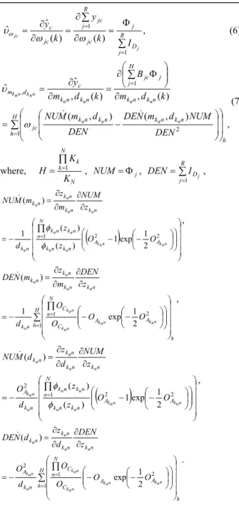
the learning rate. The gradient set of WFNN output with respect to weight set is calculated as in Eq. (4), and each gradient of WFNN output with respect to each weight is presented as in Eq. (4) to Eq. (7):
Yˆ yˆ ⎥ ⎥ ⎦ ⎤ ⎢ ⎢ ⎣ ⎡ ∂ ∂ ∂ ∂ ∂ ∂ ∂ ∂ = ∂ ∂ = ) ( ˆ ) ( ˆ ) ( ˆ ) ( ˆ ) ( ˆ ˆ k k k k k p p γY aY ωY mY dY υ , (4) n nc c a x k a y nc ∂ = ∂ = ) ( ˆ ˆ υ , (5)
, ) ( ) ( ˆ ˆ 1 1
∑
∑
= = = Φ ∂ ∂ = ∂ ∂ = R j D j jc R j jc jc c j jc I k y k y ω ω υω (6) , ) , ( ) , ( ) ( , ) ( , ˆ ˆ 1 2 1 , h H h n k n k n k n k jc n k n k H j jc j n k n k c d m DEN NUM d m N DE DEN d m M NU k d m B k d m y n n n n n n n n n n k n n k∑
∑
= = ⎟ ⎟ ⎠ ⎞ ⎜ ⎜ ⎝ ⎛ ⎟ ⎟ ⎠ ⎞ ⎜ ⎜ ⎝ ⎛ − = ∂ ⎟⎟ ⎠ ⎞ ⎜⎜ ⎝ ⎛ Φ ∂ = ∂ ∂ = & & ω υ (7) where, N N k k K K H∏
= = 1 , , , j NUM=Φ∑
= = R j Dj I DEN 1(
)
⎟ ⎟ ⎟ ⎟ ⎠ ⎞ ⎜ ⎜ ⎜ ⎜ ⎝ ⎛ ⎟⎟ ⎠ ⎞ ⎜⎜ ⎝ ⎛ ⎟ ⎠ ⎞ ⎜ ⎝ ⎛− − − = ∂ ∂ ∂ ∂ = ∏ =1 2 2 2 1 exp 1 ) ( ) ( 1 ) ( n n k n n k n n n n n n n n n A A n k n k N n kn kn n k n k n k n k n k O O z z d z NUM m z m M NU φ φ & , h H h C A A N n C n k n k n k n k n k n n k n n k n n k n n k n n n n n O O O O d z DEN m z m N DE ∑ ∏ = = ⎟ ⎟ ⎟ ⎟ ⎠ ⎞ ⎜ ⎜ ⎜ ⎜ ⎝ ⎛ ⎟⎟ ⎠ ⎞ ⎜⎜ ⎝ ⎛ ⎟ ⎠ ⎞ ⎜ ⎝ ⎛− − − = ∂ ∂ ∂ ∂ = 1 2 1 2 1 exp 1 ) ( & ,(
)
⎟ ⎟ ⎟ ⎟ ⎠ ⎞ ⎜ ⎜ ⎜ ⎜ ⎝ ⎛ ⎟⎟ ⎠ ⎞ ⎜⎜ ⎝ ⎛ ⎟ ⎠ ⎞ ⎜ ⎝ ⎛− − − = ∂ ∂ ∂ ∂ = ∏ =1 2 2 2 2 1 exp 1 ) ( ) ( ) ( n n k n n k n n n n n n n k n n n n A A n k n k N n kn kn n k A n k n k n k n k O O z z d O z NUM d z d M NU φ φ & , h H h C A A N n C n k A n k n k n k n k n n k n n k n n k n n k n n n k n n n n O O O O d O z DEN d z d N DE ∑ ∏ = = ⎟ ⎟ ⎟ ⎟ ⎠ ⎞ ⎜ ⎜ ⎜ ⎜ ⎝ ⎛ ⎟⎟ ⎠ ⎞ ⎜⎜ ⎝ ⎛ ⎟ ⎠ ⎞ ⎜ ⎝ ⎛− − − = ∂ ∂ ∂ ∂ = 1 2 1 2 2 1 exp ) ( & .3. PATH TRACKING CONTROL FOR MOBILE
ROBOT USING THE WFNN
3.1 Dynamic model of mobile robot
x y World Coordinate r b Drivin g W heel Caster , θ ) ( yx
Fig. 1 Mobile robot model and world coordinate The mobile robot used in this paper is composed of two driving wheels and four casters. And it is fully described by a three dimensional vector of generalized coordinates constituted by the coordinates of the midpoint between the two
driving wheels, and by the orientation angle with respect to a fixed frame as shown in Fig. 1. The equation for motion dynamics is as follows: ⎥ ⎥ ⎥ ⎥ ⎥ ⎥ ⎥ ⎦ ⎤ ⎢ ⎢ ⎢ ⎢ ⎢ ⎢ ⎢ ⎣ ⎡ + + + ⎥ ⎥ ⎥ ⎦ ⎤ ⎢ ⎢ ⎢ ⎣ ⎡ = ⎥ ⎥ ⎥ ⎦ ⎤ ⎢ ⎢ ⎢ ⎣ ⎡ + + + k k k k k k k k k k k k k sin d cos d Y X Y X δθ δθ θ δ δθ θ δ θ θ ) 2 ( ) 2 ( 1 1 1 , (8)
where, and are linear velocity and angular velocity, respectively, and and are two incremental distances of two driving wheels and distance between these two wheels, respectively. In this model, the control input vector is represented by d δ δθ , r d dl b
[
] [
T]
T du d u θ =δ δθ = U .3.2 The direct adaptive control system using the WFNN In our control system, the direct adaptive control system is designed using the WFNN structure. The purpose of our control system is to minimize the state error
between the reference trajectory and the controlled trajectory ) , , (ex ey eθ E ) , , ( r r r r x y θ Y ) , , (x yθ
Y of a mobile robot. For this purpose, the parameters of WFNN are trained via the GD method. The overall control system is shown in Fig. 2. WFNN controller calculates the control input by training the inverse dynamics of plant iteratively. But, the updating of parameters of WFNN through the variation rate in the GD method cannot be calculated directly. So, we train the parameters of a WFNN through the transformation of the output error of plant.
[
]
T du u θ = U ) , ( Yγ J Mobile Robot ) , (δdδθ uc ) , , (xyθ trajectory controlled Y ) , , (r r r rx y trajectory reference θ Y + − ∑ Gradient Descent Method and Lyapunov Stability Analysis ) ,e ,e (e error state θ y x EThe Direct Adaptive Controller Based on
WFNN
Feedforward Jacobian of Mobile Robot Updating the parameters
of WFNN
Fig. 2 Direct adaptive control system
In this structure, inputs are composed of errors between the reference trajectory and the controlled trajectory, and outputs are control variables. Each control variable is as follows:
, , 1 3 1 1 3 1 1 3 1 1 3 1 ∑ ∑ ∑ ∑ ∑ ∑ ∑ ∑ = = = = = = = = Φ + = + = Φ + = + = R j j j n n n R j j n n n R j jd j n nd n R j jd n nd n d B e a y e a u B e a y e a u θ θ θ θ θ (9) where, ∑ ∏ ∏ = = = ⎟ ⎟ ⎟ ⎠ ⎞ ⎜ ⎜ ⎜ ⎝ ⎛ ⎟ ⎟ ⎟ ⎠ ⎞ ⎜ ⎜ ⎜ ⎝ ⎛ ⎟ ⎟ ⎠ ⎞ ⎜ ⎜ ⎝ ⎛ − − ⎟ ⎟ ⎟ ⎠ ⎞ ⎜ ⎜ ⎜ ⎝ ⎛ ⎟ ⎟ ⎠ ⎞ ⎜ ⎜ ⎝ ⎛ − − ⎟ ⎟ ⎠ ⎞ ⎜ ⎜ ⎝ ⎛ ⎟ ⎟ ⎠ ⎞ ⎜ ⎜ ⎝ ⎛ − − = Φ R j j n kn n k n n kn n k n n k n k n jc j jc n n n n n n d m e d m e d m e B 1 3 1 2 3 1 2 2 1 exp 2 1 exp ω and }. , {dθ c=
raining Procedure :
g the parameters of WFNN is to
t function so as to train a T
The purpose of trainin
minimize the state errors E(ex,ey,eθ). To do this, we present the following training procedure:
· Definition of the following cos
WFNN controller based on direct adaptive control technique: ) ) ( ) ( ) (( 1 − 2+ − 2+ θ −θ 2 = xr x yr y r C . (10) 2
· Calculation of the partial derivative of the cost function with respect to the parameter set of a WFNN controller:
, ) ( p p γ U∂ p y p x p p p p u J e y e x e γ U E U γ U U γ U U γ γ γ γ ∂ ∂ − = ∂ ∂ ∂ − ∂ ∂ ∂ ∂ − ∂ ∂ ∂ ∂ − = ∂ ∂ ∂ ∂ θ θ (11) y x e y e x e C =− ∂ − ∂ − ∂ ∂ θ θ where, ex=xr−x, ey =yr−y eθ =θr−θ and U Y ∂ ∂ = ) (u
J is the feedforward Jacobian of a mobile robot and is as follows: . 1 0 ) 2 ( 2 ) 2 ( ) 2 ( 2 ) 2 ( ) ( 1 − = ⎥ ⎥ ⎥ ⎥ ⎥ ⎥ ⎥ ⎦ ⎤ ⎢ ⎢ ⎢ ⎢ ⎢ ⎢ ⎢ ⎣ ⎡ + + + − ∂ + = k k k k k k k k k k k k cos d sin sin d cos u J θ θ δθ θ δ δθ θ δθ θ δ θ θ (12)
The partial derivative of the control input with respect to the parameters of a WFNN controller can be calculated by using Eqs. (13) and (14).
U
· Updating of the parameters of WFNN via the following iterative GD method: , ) ( ) ( ) ( ) ( ) ( ) 1 ( p p p p p p p u J k C k k k k γ U E γ γ γ γ γ γ ∂ ∂ − = ∂ ∂ − = ∆ + = + η η (12)
where, η is the learning rate of a WFNN.
From Eqs (12) and (13), each gradient of the controller output with respect to each weight is presented as follows:
c u h H h n k n k n k n k jc n k n k H j jc j n k n k c R j D j jc R j jc jc c n nc c DEN NUM d m N DE DEN d m M NU k d m B k d m u I k y u e a u n n n n n n n n j ∑ ∑ ∑ ∑ = = = = ⎟ ⎟ ⎠ ⎞ ⎜ ⎜ ⎝ ⎛ ⎟ ⎟ ⎠ ⎞ ⎜ ⎜ ⎝ ⎛ − = ∂ ⎟⎟ ⎠ ⎞ ⎜⎜ ⎝ ⎛ Φ ∂ = ∂ ∂ Φ = ∂ ∂ = ∂ ∂ = ∂ ∂ 1 2 1 1 1 ) , ( ) , ( ) ( , ) ( , ) ( , & & ω ω ω , (13)
and the detailed description is shown in Eq. (7).
4. STABILITY OF THE WFNN CONTROLLER
In the update rule of Eq. (3), selection of the values for the learning rate η has the significant effect on the control performance. Generally, if η is too big, the system is
unstable. And for the small η, although the convergence is guaranteed, the control speed very slow. Therefore, in order to train the WFNN effectively, adaptive learning rates, which guarantee the fast convergence and stability, must be derived. In this subsection, the specific learning rates for the type of network weights are derived based on the convergence analysis of a discrete type Lyapunov function.
Theorem 1: Let p,c
is
η be the learning rate for the output nd are defined
c u
influenced by weight vector γ of the WFNN. p Gp,c(k) a
) ( max , ,c k p G as ) ( ) ( k k u p c γ ∂ ) ( ,c k p G = ∂ and ) ( max ) ( , max , ,c k k pc k p G
G ≡ , respectively, and ⋅ is the Euclidean norm in ℜn. Here, subscript p and denote each weight and outpu espectively. Then the convergence is guaranteed if p,c c t, r η is chosen as follows:
(
2)
, 2 , 2 , 2 max , , , ) ( 2 0 c c y c x c p c p J J J k θ η + + < < G . (14) Proof:nalysis, a discrete type Lyapunov function is selected In this a as ) ( 2 1 ) (k V = ETEk , (15) where, is and Lyapu ) (k
E the difference between the desired state )
(k
r
Y the output state Y(k). Then, the change of nov function is obtained by
)) ( ) 1 ( ) ( ) 1 ( ) ( ) 1 ( ( 2 1 ) ( ) 1 ( ) ( 2 2 2 2 2 2 k e k e k e k e k e k e k V k V k V y y x x + − + + − + θ + − θ = − + = ∆ ,(16) where, ( ) ) ( ) ( ) ( ) 1 ( ) ( k k k e k e k e k e p T p x x x x γ ∆γ ⎥ ⎥ ⎦ ⎤ ⎢ ⎢ ⎣ ⎡ ∂ ∂ ≈ − + = ∆ , ) ( ) ( ) ( ) ( k k k e k e p T p y y γ ∆γ ⎥ ⎥ ⎦ ⎤ ⎢ ⎢ ⎣ ⎡ ∂ ∂ ≈ ∆ , ( ) ) ( ) ( ) ( k k k e k e p T p γ γ ⎥⎥⎦ ∆ ⎤ ⎢ ⎢ ⎣ ⎡ ∂ ∂ ≈ ∆ θ θ .
From Eqs. (27), (28) and (29), ∆γp(k) is defined as
⎥ ⎥ ⎦ ⎤ ⎢ ⎢ ⎣ ⎡ ∂ ∂ ⎟⎟ ⎠ ⎞ ⎜⎜ ⎝ ⎛ ∂ ∂ + ∂ ∂ + ∂ ∂ = ∂ ∂ − = ∆γ (k) η C ) ( ) ( ) ( ) ( ) ( ) ( ) ( ) ( ) ( ) ( ) ( ) ( , , k k u k u k k e k u k y k e k u k x k e k p c c c y c x c p p c p p γ γ θ η θ , (17)
and the error difference can be represented by
, ) ( ) ( ) ( ) ( ) ( ) ( ) ( ) ( ) ( ) ( ) ( ) ( ) ( ) ( ) ( ) ( ) ( ) ( ) ( ) ( ) ( ) ( ) ( ) ( ) ( ) ( ) ( ) ( ) ( ) ( ) ( ≈⎢⎡ ∂ ⎥⎤∆ ∆e k e k pk T x x γ ) ( 2 , , ⎟⎟ ⎠ ⎞ ⎜⎜ ⎝ ⎛ ∂ ∂ + ∂ ∂ + ∂ ∂ ∂ ∂ ∂ ∂ − = ⎥ ⎥ ⎦ ⎤ ⎢ ⎢ ⎣ ⎡ ∂ ∂ ⎟⎟ ⎠ ⎞ ⎜⎜ ⎝ ⎛ ∂ ∂ + ∂ ∂ + ∂ ∂ ∂ ∂ ⎥ ⎥ ⎦ ⎤ ⎢ ⎢ ⎣ ⎡ ∂ ∂ − = ⎥⎦ ⎢⎣∂ k u k k e k u k y k e k u k x k e k u k x k k u k k u k u k k e k u k y k e k u k x k e k u k x k k u k c c y c x c p c c p p c c c y c x c p c T p c p θ η θ η θ θ γ γ γ γ (18) h
w ere, )∆ey(k and have the same description. Let a elem feed ) (k eθ ∆ c s
J , be ent of the forward Jacobian for the state of obile robot with respect to the control input, where, subscript
a m
s and c denote one state among three state of a
mobile rob t and the control input u , respectively. From Eqs. c
(16) - (18), V(k) o
[
]
(
)
(
)
(
)
(
)
(
)
(
)
(
)
(
(
() () ())
(). ) ( ) ( 2 1 1 ) ( ) ( ) ( ) ( ) ( ) ( ) ( ) ( ) ( ) ( 2 1 ) ( ) ( ) ( ) ( ) ( ) ( ) ( ) ( ) ( ) ( ) ( 2 1 ) ( ) ( ) ( ) ( ) ( ) ( ) ( ) ( ) ( ) ( ) ( 2 1 ) ( ) ( ) ( ) ( ) ( ) ( ) ( 2 1 ) ( ) ( ) ( 2 1 ) ( ) ( ) ( 2 1 ) ( ) ( ) ( )) ( ) ( ( ) ( )) ( ) ( ( ) ( )) ( ) ( ( 2 1 ) ( ) 1 ( ) ( 2 , , , 2 , 2 , 2 , 2 , 2 , 2 , , , , , , , 2 , , , , 2 , , , , , 2 , , , , 2 , , , , , 2 , , , , 2 , 2 2 2 2 2 2 k J k e J k e J k e J J J k k u k k u J k e J k e J k e J k e J k e J k e J k k u k e J k e J k e J k e J k k u J k e J k e J k e J k k u k e J k e J k e J k e J k k u J k e J k e J k e J k k u k e J k e J k e J k e J k k u k e k e k e k e k e k e k e k e k e k e k e k e k e k e k e k e k e k e k V k V k V c c y y c x x c c y c x p c c p p c c p c c y y c x x c c y y c x x c p c c c y y c x x c p c c p c c y y c x x c y p c y c c y y c x x c y p c c p c c y y c x x c x p c x c c y y c x x c x p c c p y y y x x x y y y x x x ρ η η η η η θ θ θ θ θ θ θ θ θ θ θ θ θ θ θ θ θ θ θ θ θ θ θ θ θ θ + + − = ⎥ ⎥ ⎥ ⎦ ⎤ ⎢ ⎢ ⎢ ⎣ ⎡ ⎟⎟ ⎟ ⎠ ⎞ ⎜⎜ ⎜ ⎝ ⎛ + + ∂ ∂ − ∂ ∂ + + − = ⎥ ⎥ ⎦ ⎤ ⎢ ⎢ ⎣ ⎡ + + ∂ ∂ − ⋅ + + ∂ ∂ − ⎥ ⎥ ⎦ ⎤ ⎢ ⎢ ⎣ ⎡ + + ∂ ∂ − ⋅ + + ∂ ∂ − ⎥ ⎥ ⎦ ⎤ ⎢ ⎢ ⎣ ⎡ + + ∂ ∂ − ⋅ + + ∂ ∂ − = ⎥⎦ ⎤ ⎢⎣ ⎡ + ∆ ∆ + ⎥⎦ ⎤ ⎢⎣ ⎡ + ∆ ∆ + ⎥⎦ ⎤ ⎢⎣ ⎡ + ∆ ∆ = − ∆ + + − ∆ + + − ∆ + = − + = ∆ γ γ γ γ γ γ γ γ)
Let us define Gp,c(k) and Gp,c,max(k) as
) ( ) ( ) ( , k k u k p c c p γ G ∂ ∂
= and Gp,c,max(k)≡maxk Gp,c(k) , respectively. Since
(
)
(
)
(
)
0 ) ( 2 1 1 ) ( ) ( ) ( ) ( 2 1 1 ) ( ) ( 2 1 1 ) ( ) ( 2 , 2 , 2 , 2 max , , , 2 , , 2 max , , 2 , 2 , 2 , 2 , 2 max , , , 2 , , 2 , 2 , 2 , 2 , , 2 , , > ⎥⎦ ⎤ ⎢⎣ ⎡ − + + ≥ ⎥ ⎥ ⎥ ⎦ ⎤ ⎢ ⎢ ⎢ ⎣ ⎡ + + − = ⎥⎦ ⎤ ⎢⎣ ⎡ − + + = c c y c x c p c p c p c p c p c c y c x c p c p c p c p c p c c y c x c p c p c p c p J J J k k k J J J k k k J J J k k k θ θ θ η η η η η η ρ G G G G G G G G ,(19) we obtain(
2)
, 2 , 2 , 2 max , , , ( ) 2 0 c c y c x c p c p k J J J θ η + + < < G ■ Q.E.D. (20) Remark 1: The convergence is guaranteed as long as Eq. (19) is satisfied, i.e.:(
0 ) ( 2 1 1 , 2,,max 2, 2, 2, ,c⎢⎣⎡ − pc pc xc+ yc+ c⎤⎥⎦> p η k J J Jθ η G)
. (21)The maximum learning rate, which guarantees the fast convergence, can be obtained as
(
)
1 ) ( 2 , 2 , 2 , 2 max , , ,c pc xc+ yc+ c = p k J J Jθ η G , i.e.:(
2)
, 2 , 2 , 2 max , , max , , ) ( 1 c c y c x c p c p J J J k θη
+ + = G , (22) which is the half of the upper limit.Theorem 2: Let ηp,c={ηa,c,ηω,c,ηm,c,ηd,c} be the learning rate set for the weight set, of WFNN, and
is defined as the gradient set, }, , , , {a ω d m γ= ) ( ,c k p G , ) ( ) ( , ) ( ) ( , ) ( ) ( , ) ( ) ( ⎭ ⎬ ⎫ ⎩ ⎨ ⎧ ∂ ∂ ∂ ∂ ∂ ∂ ∂ ∂ k k u k k u k k u k k uc c c c d m ω a of WFNN output
with respect to the weight set. Then the convergence is guaranteed if c u c p, η is chosen as
(
)
(
)
(
)
(
2)
(
)
. 0 ) ( , 2 0 ) ( , 2 0 ) ( , 2 0 ) ( max 2 , 2 , 2 , 2 2 min max 2 , 2 max , max 2 , 2 , 2 , 2 2 min 2 max , 2 , 2 , 2 , 2 max 2 , 2 , 2 , 2 , 2 max , c c y c x n k n k A jc c d c c y c x n k jc c m c c y c x B c c c y c x n c a J J J DEN d H DEN O H C d J J J DEN d H DEN H C c J J J O R b J J J e N a n n n j θ θ θ ω θ ω η ω η η η + + ⎟ ⎟ ⎟ ⎠ ⎞ ⎜ ⎜ ⎜ ⎝ ⎛ + < < + + ⎟ ⎟ ⎟ ⎠ ⎞ ⎜ ⎜ ⎜ ⎝ ⎛ + < < + + < < + + < < (23) Proof : (a)Let us define Ga,c,max(k) as Ga,c,max(k)≡maxk Ga,c(k) . Then from Eq. (20), we obtain
(
2)
, 2 , 2 , 2 max , , , ) ( 2 0 c c y c x c a c a J J J k θ η + + < <G . And from the
definition of Theorem 1, the maximum condition can be obtained as max , max ) ( ) ( max ) ( max k n nc c k c a k Ne k a k u k = ≤ ∂ ∂ = E G . Thus 2 2max max , ,c ( ) n a k =Ne G ,
where is the -th input value of WFNN and is the number of input. The rest of proof is shown in the Appendix
n
e n N
■ Q.E.D.
Remark 2: The maximum learning rates of WFNN, which guarantee the fast convergence, are as shown in Eq. (24).
(
)
(
)
(
)
(
)
(
)
. 1 , 1 , 1 , 1 max 2 , 2 , 2 , 2 2 min max 2 , 2 max max , , max 2 , 2 , 2 , 2 2 min 2 max max , , 2 , 2 , 2 , 2 max 2 max , , 2 , 2 , 2 , 2 max max , , c c y c x n k n k A jc c d c c y c x n k jc c m c c y c x B c c c y c x n c a J J J DEN d H DEN O H C J J J DEN d H DEN H C J J J O R J J J e N n n n j θ θ θ ω θ ω η ω η η η + + ⎟ ⎟ ⎟ ⎠ ⎞ ⎜ ⎜ ⎜ ⎝ ⎛ + = + + ⎟ ⎟ ⎟ ⎠ ⎞ ⎜ ⎜ ⎜ ⎝ ⎛ + = + + = + + = (24)5. SIMULATIONS
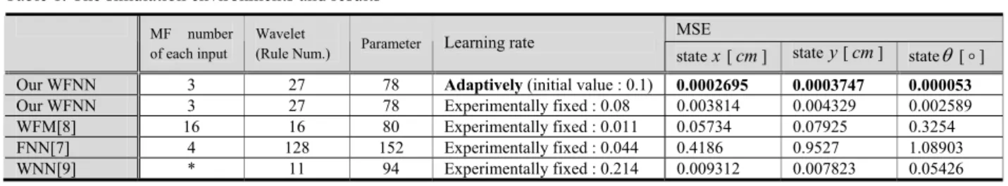
In this section, we present simulation results to validate the control performance of the proposed WFNN controller for the path tracking of mobile robots. Generally, the characteristic of network structure as a controller is very susceptible to several simulation environments such as the initial value of network weight, the sampling time, the learning rate, etc. In this computer simulation, the initial values of network weight are randomly determined and the sampling time of control procedure is 0.01sec. In the update rule of GD method, selection of the values for the learning rate η has the significant effect on the control performance. So, in our control system, the learning rates are adaptively determined to rapidly minimize the state errors. The inputs of controller are three state errors, . The simulation environments and results are as shown in Table 1. This simulation considers the tracking of a trajectory generated by the following displacements: ) , , (ex ey eθ E
Table 1. The simulation environments and results ) 20 15 ( sec / 0 sec, / 20 ) 15 10 ( sec / 3 . 59 sec, / 30 ) 10 5 ( sec / 3 . 59 sec, / 30 ) 5 0 ( sec / 0 sec, / 20 ≤ < ° = = ≤ < ° − = = ≤ < ° = = ≤ < ° = = t velocity Angular cm d velocity Linear t velocity Angular cm d velocity Linear t velocity Angular cm d velocity Linear t velocity Angular cm d velocity Linear δθ δ δθ δ δθ δ δθ δ 0 50 100 150 -20 -10 0 10 20 30 40 50 60
70 Tracking result for mobile robot using WFNN controller
X position(cm) Y po si tion (c m ) Reference trajectory Controlled trajectory
Fig. 3 Controlled path using a WFNN controller
0 2 4 6 8 10 12 14 16 18 20 -0.2 -0.1 0 0.1 0.2 Time(sec) er ro r x( cm ) Tacking errors 0 2 4 6 8 10 12 14 16 18 20 -0.1 -0.05 0 0.05 0.1 0.15 Time(sec) erro r y (c m ) 0 2 4 6 8 10 12 14 16 18 20 -15 -10 -5 0 5 10 Time(sec) er ro r θ( ang le )
Fig. 4 Path tracking errors
0 2 4 6 8 10 12 14 16 18 20
0 2000
4000 Adaptive learning rates
Time step a f or u 1 0 2 4 6 8 10 12 14 16 18 20 0 2000 4000 Time step a f or u2 0 2 4 6 8 10 12 14 16 18 20 0 1 2 Time step w f or u 1 0 2 4 6 8 10 12 14 16 18 20 0 1 2 Time step w f or u 2 0 2 4 6 8 10 12 14 16 18 20 0 0.02 0.04 Time step m f or c on tro l i np ut s 0 2 4 6 8 10 12 14 16 18 20 0 0.5 1x 10 -3 Time step d fo r c ont ro l i np ut s
Fig. 5 Adaptive learning rates for the WFNN weights Figure 3 shows the reference path and controlled path of a mobile robot using a WFNN controller. And Figs. 4 and 5 show the control errors for path tracking of a mobile robot and the adaptive learning rates for the fast convergence and
MSE
MF number of each input
Wavelet
(Rule Num.) Parameter Learning rate statex[cm] statey cm[ ] stateθ [ ] o
Our WFNN 3 27 78 Adaptively (initial value : 0.1) 0.0002695 0.0003747 0.000053
Our WFNN 3 27 78 Experimentally fixed : 0.08 0.003814 0.004329 0.002589
WFM[8] 16 16 80 Experimentally fixed : 0.011 0.05734 0.07925 0.3254
FNN[7] 4 128 152 Experimentally fixed : 0.044 0.4186 0.9527 1.08903
WNN[9] * 11 94 Experimentally fixed : 0.214 0.009312 0.007823 0.05426
stability, respectively. As a result, if the control errors are changed then the learning rates are changed too for the fast convergence and accuracy. In our simulations, we use the mean squared error(MSE) as the tracking performance for comparison of performance with the FNN, the WFM and the WNN controllers. The simulation results are as shown in Table 1. From these figures and Table 1, we confirm that the WFNN controller works better than other controllers that use the FNN, the WFM and the WNN respectively, although the tracking errors are occurred in case that the direction is changed. In this comparison, the network structure such as the number of membership function, the number of rule and the learning rate, is experimentally determined via many simulations.
6. CONCLUSION
In this paper, we have proposed a WFNN based direct adaptive control scheme for the solution of the tracking problem of mobile robots. In our control system, we have designed a FNN structure based on wavelet that merges the advantages of neural network, fuzzy model and wavelet transform as a controller. The control signals were directly obtained to minimize the difference between the reference track and the pose of a mobile robot via the GD method. In addition, an approach that has used adaptive learning rates for the training of WFNN controller was driven via a Lyapunov stability analysis to guarantee the fast convergence, that is, learning rates were adaptively determined to rapidly minimize the state errors of a mobile robot. Finally, to evaluate the performance of the proposed direct adaptive control system using WFNN, we have compared the control results of the WFNN controller with those of the FNN, the WNN and the WFM controllers. As a result, we have confirmed that our WFNN controller works better than the FNN, the WNN and the WFM controllers, although the tracking errors are occurred in case that the direction is changed.
APPENDIX
Proof (b) of Eq. (23):
Let us define Gω,c,max(k) as Gω,c,max(k)≡maxk Gω,c(k) . And then from Eq. (13) and the definition of Theorem 1, the gradient of WFNN output uc with respect to weight ωjc
can be written as
∑
= Φ = ∂ ∂ = R j D j jc c c j I k u k 1 , ( ) ω ( ) ω G , then B B B R j j j B R j j j c k = O j ≤ O j ≤O j ≤ O ∑ ∑ = =1 1 , ( ) µ µ µ µ ω G .Since 1 1 < ∑ = R j j j µ µ and R R j j j < ∑ =1µ µ , we obtain max ,c(k) ≤ R OB ≤ROBj ω
G and have the
maximum condition as follows: 2 max 2 2 max , ,c (k)=R OBj ω G . (A1) Hence, from Theorem 1 and Eq. (A1), (b) of Theorem 2 follows ■ Q.E.D.
Proof (c) and (d) of Eq. (23):
Let us define
G
m,d,c−out(
k
)
as)
(
max
)
(
, , , ,dc outk
k mdck
mG
G
−≡
. And then from Eq. (13) and the definition of Theorem 1, the gradient of WFNN output with respect to weight and can be written asc
u
mknn dknn . ) , ( ) , ( ) ( , ) ( 1 2 1 , , , , ∑ ∑ = = ⎟ ⎟ ⎠ ⎞ ⎜ ⎜ ⎝ ⎛ ⎟ ⎟ ⎠ ⎞ ⎜ ⎜ ⎝ ⎛ − = ∂ Φ ∂ = H h n k n k n k n k jc H j k n k n j jc c d m DEN NUM d m N DE DEN d m M NU k d m B k n n n n n n & & ω G Since(
)
1 2 1 exp 1 ) ( 2 2 ⎟< ⎠ ⎞ ⎜ ⎝ ⎛− − = jn jn jn jn z z z φ& and 1 2 1 exp 2 1 p x e 2 2 ⎟< ⎠ ⎞ ⎜ ⎝ ⎛− − = ⎟ ⎠ ⎞ ⎜ ⎝ ⎛− zjn zjn zjn & , we obtain , ) ( ) ( ) ( 2 min max 1 2 1 , ⎟ ⎟ ⎟ ⎠ ⎞ ⎜ ⎜ ⎜ ⎝ ⎛ + ≤ ⎟ ⎟ ⎠ ⎞ ⎜ ⎜ ⎝ ⎛ + ⎟ ⎟ ⎠ ⎞ ⎜ ⎜ ⎝ ⎛ ≤ ∑ ∑ = = DEN d H DEN H DEN NUM m N DE DEN m M NU k n k jc H j n k jc H j n k jc c m n n n ω ω ω & & G and(
)
. ) ( ) ( ) ( 2 min max 2 , max 1 2 1 , ⎟ ⎟ ⎟ ⎠ ⎞ ⎜ ⎜ ⎜ ⎝ ⎛ + ≤ ⎟ ⎟ ⎠ ⎞ ⎜ ⎜ ⎝ ⎛ + ⎟ ⎟ ⎠ ⎞ ⎜ ⎜ ⎝ ⎛ ≤ ∑ ∑ = = DEN d H DEN O H DEN NUM d N DE DEN d M NU k n k n k A jc H j n k jc H j n k jc c d n n n n ω ω ω & & GTherefore, we obtain each maximum condition as follows: 2 2 min 2 max 2 , ( ) ⎟ ⎟ ⎟ ⎠ ⎞ ⎜ ⎜ ⎜ ⎝ ⎛ + = − DEN d H DEN H k n k jc out c m n ω G , (A2)
(
)
2 2 min max 2 , 2 max 2 , ( ) ⎟ ⎟ ⎟ ⎠ ⎞ ⎜ ⎜ ⎜ ⎝ ⎛ + = − DEN d H DEN O H k n k n k A jc out c d n n ω G . (A3)While the weight a and have an effect on only one connected output, the weight and have an effect on all output. Therefore, for the convergence according to the effect of the weight and d , the additional expansion is
needed. Let us define as
ω m d m ) ( 2 max , , ,dc k m G
(
)
. ) ( max ) ( 2 , 2 , 2 , 2 , , 2 max , , ,dc k mdcout xc yc c m k ≡ G − k J +J +Jθ G Hereis the maximum condition for each output according to the effect of the weight and
is the maximum condition for output . Then we obtain ) ( 2 , ,dc out k m − G
u
c } , {m d ) ( 2 max , , ,dc k m G U(
2)
max , 2 , 2 , 2 , , 2 max , , ,dc ( ) mdcout( ) xc yc c m k ≤ CG − k J +J +Jθ G , thus(
)
max 2 , 2 , 2 , 2 2 min 2 max 2 max , , ( ) xc yc c n k jc c m J J J DEN d H DEN H C k n θ ω + + ⎟ ⎟ ⎟ ⎠ ⎞ ⎜ ⎜ ⎜ ⎝ ⎛ + = G , (A4)(
)
(
)
max 2 , 2 , 2 , 2 2 min max 2 , 2 max 2 max , , ( ) xc yc c n k n k A jc c d J J J DEN d H DEN O H C k n n θ ω + + ⎟ ⎟ ⎟ ⎠ ⎞ ⎜ ⎜ ⎜ ⎝ ⎛ + = G . (A5)Therefore, if the maximum condition Eqs. (A2) and (A3) are substituted by Eqs. (A4) and (A5), respectively, from Theorem 1, Eqs. (A4) and (A5), (c) and (d) of Theorem 2 follow ■ Q.E.D.
REFERENCES
[1] X. Yang, K. He, M. Guo, and B. Zhang, "An intelligent predictive control approach to path tracking problem of autonomous robot," Proc. of IEEE Conf. on Systems, Man, and Cybernetics, Vol. 4, pp. 350-355, 1998.
[2] Z. P. Jiang and H. Nijmeijer, "Tracking control of mobile robots: a case study in backstepping," Automatica, Vol. 33. No. 7, pp. 1393-1399, 1997.
[3] J. M. Yang and J. H. Kim, "Sliding mode motion control of nonholonomic mobile robots," IEEE Control Systems, Vol. 19, No. 2, pp. 15-23, 1990.
[4] M. L. Corradini, G.. Ippoliti, S. Longhi and S. Michelini, "Neural networks inverse model approach for the tracking problem of mobile robot," Proc. of RAAD, pp. 17-22, 2000. [5] M. L. Corradini, G. Ippoliti, and S. Longhi, "The tracking problem of mobile robots: experimental results using a neural network approach," Proc. of WAC, pp. 33-37, 2000.
[6] T. Hasegawa, S. Horikawa, T. Furuhashi and Y. Uchikawa, "On design of adaptive fuzzy neural networks and description of its dynamical behavior," Fuzzy Sets and Systems, Vol. 71, No. 1, pp. 3-23, 1995.
[7] J. T. Choi and Y. H. Choi, " Fuzzy neural network based predictive control of chaotic nonlinear systems," IEICE Trans. on Fundamentals, Vol. E87-A, No. 5, pp. 1270-1279, 2004. [8] C. K. Lin and S. D. Wang, "Fuzzy modeling using wavelet transforms," Electronics Letters, Vol. 32, pp. 2255-2256, 1996.
[9] Y. Oussar, I. Rivals, L. Personnaz and G. Dreyfus, "Training wavelet networks for nonlinear dynamic input-output modeling," Neurocomputing, Vol. 20. pp. 173-188, 1998.
[10] J. S. Oh and Y. H. Choi, "Path tracking control using a wavelet based fuzzy neural network for mobile robots," International Journal of Fuzzy Logic and Intelligent Systems, Vol. 4, No. 1, pp. 111-118, 2004.
[11] S. Mallat, "A theory for multiresolution signal decomposition: the wavelet transform," IEEE Trans. on
Pattern Anal. Mach. Intelligence, Vol. 11, No. 7, 674-693,