Multigrid Methods for Improving the Variational Data
Assimilation in Numerical Weather Prediction
By Youn-Hee Kang1?, Do Young Kwak,1and Kyungjeen Park2,
1Department of Mathematical Science, KAIST, Daejeon, Republic of Korea;2Numerical Model Development Division, Korea Meteorological Administration, Seoul, Republic of Korea
(Manuscript received 23 November 2012)
ABSTRACT
Two conditions are needed to solve Numerical Weather Prediction models: initial condition and boundary condition. The initial condition has especially an important bearing on the model performance. To get a good initial condition, many data assimi-lation techniques have been developed for the meteorological and the oceanographical fields. Currently, the most commonly used technique for operational applications is the 3 dimensional or 4 dimensional variational data assimilation method. The numerical method used for the cost function minimizing process is usually an iterative method such as the conjugate gradient. In this paper, we use the multigrid method (MG) based on the cell centered finite difference (CCFD) on the variational data assimilation to improve the performance of the minimization procedure for 3D Var data assimilation. 1 Introduction
Numerical Weather Prediction models consist of equa-tions based on the laws of physics, fluid motion, and chem-istry that govern the atmospheric flow. Such a model is a very big and complex system having various scale domains from meter to global areas. To solve this system, there are two necessary conditions, initial and boundary condition. The initial condition has an especially important bearing on the model performance. (Downton (1998); Richardson (1998))
If there is enough observational data provided by obser-vation of the true states, the initial field is given by interpo-lating the observation data. However, in most cases observa-tional data is inhomogeneous and not sufficient, so the prob-lem is under-determined although it can be over-determined locally in data-dense areas. In order to overcome this prob-lem, it is necessary to apply some background information in the form of an a priori estimate of the model state. Physi-cal constraints are also a help. The background information is usually obtained from the model output at previous time steps. Then the initial conditions are obtained by combining short model forecasts (called a background field) with the observational data. This process is called a data assimila-tion, and the output field of a data assimilation is called an analysis field.
Many data assimilation techniques have been developed for meteorology and oceanography. Currently, the most com-monly used techniques for operational applications are 3 or 4 dimensional variational data assimilation methods (3D-Var or 4D-Var). The variational data assimilation methods
con-? Corresponding author.
e-mail: unimoon@kaist.ac.kr. current address: Numerical Model Development Division, KMA, Seoul, Korea
sist of the following processes: the generation of background error covariance to determine the spatial spreading and rela-tion of variables of observarela-tional informarela-tion; preprocessing of observational data and the observation operator (to in-terpolate the model value on the observation position with model values on the model grid position and to transform the model variables to observational variables); and minimizing of the cost function. The last one, the cost function minimiz-ing process, finds the maximum likelihood point by usminimiz-ing the error distributions of the observation field and background field. Under the condition that the error distributions are normal, the cost function has a quadratic form. Then the minimum of the cost function is found at a stationary point where the gradient of the cost function vanishes. The most popular numerical methods applied to the cost function min-imizing process are usually iterative methods, such as the conjugate gradient (CG) method and the Limited Memory BFGS (L-BFGS) method, etc.
The purpose of this paper is to improve the performance of the iterative minimization procedure. We begin with a few considerations: The first thing is that the observational data for data assimilation are rapidly increasing. Hence a faster minimization procedure is needed. The second thing is the convergence of long wave data. It is well-known that relaxation methods such as Jacobi or Gauss-Seidel meth-ods have a smoothing property. The convergence speed of general relaxation methods depends on long wavelength er-ror convergence because short wave length erer-rors on a fine grid decrease faster than wavelength errors (Briggs (2000)). This phenomenon matches the fact that for given observa-tion systems, data-sparse regions provide long wave infor-mation and data-dense regions provide both long wave and short wave information. Thus it would be nice if one could design a method which can extract long wave information over the data-sparse regions and shortwave information over
data-dense regions (Li (2010)), which is a motivation of the multigrid method.
Multigrid methods for solving linear system utilizes the smoothing property of the relaxation schemes, and using the nested grids one can retrieve the long wave information without much affecting shortwave information. In this paper, we apply multigrid methods based on cell centered finite differences (CCFD) on the Variational Data Assimilation to overcome above problems in the iterative minimization procedure.
Multigrid methods are well-known techniques for solv-ing elliptic partial differential equations (PDE), (see Briggs (2000) and references therein) but it seems that their use for Data Assimilation problems was first initiated in Li (2008), Li (2010). However, our work in this study is different from them in a number of ways. First, we interpret the data as-similation problem as an elliptic (diffusion type) partial dif-ferential equation discretized by the CCFD so that the geo-metric data (observation point, velocity, temperature, etc.) carry over to the model equation accurately. (The CCFD is known to conserve mass locally, so it has higher accu-racy than the finite difference method which is based on the point values). Even though one cannot tell what this PDE looks like, we can define the prolongation and restriction op-erators by mimicking the diffusion process. A homogenous boundary condition was assumed and the necessary data near the boundary were obtained by reflection or extrapo-lation. Second, we explain why the Jacobi relaxation can be implemented more efficiently than the Gauss-Seidel (section 3.2.4). These are different from the conventional multigrid methods because in our minimization problem, the matrix entries are not explicitly given. Furthermore, we describe the concrete data transfer operator between a fine grid and a coarser grid, which is based on the geometry (See Figure 5).
Near the completion of our paper, we found that Grat-ton et al. (GratGrat-ton (2013)) also used a multigrid method, but they used it only to perform the matrix vector product of the background covariance matrix B by solving the re-lated heat equation. Hence their procedure is quite different from ours.
This paper is organized as follows. In section 2, we re-view the basic concept of MG methods and some basic tech-niques. In section 3, we describe MG algorithms for use in a minimization process in incremental 3D-Var. In section 4, we show some numerical comparisons of an analysis produced by CG and by MG. Lastly, section 5 gives our concluding remarks.
2 Brief introduction of Multigrid Methods
Traditional relaxation methods, such as Jacobi, Gauss -Seidel or SOR, have a common property, called a ’smoothing property’. This property makes such methods very effective at eliminating the high-frequency or oscillatory components of the error, while leaving the low-frequency or less oscil-latory components relatively unchanged (Fig.1). The con-vergence speed of general iterative methods depends mainly on the long wavelength error convergence. That means that these methods have a correct solution from the dense (short wavelength) structure but the convergence depends on the
coarse (long wavelength) structure. One way to improve such a relaxation scheme, at least in the early stages, is to use a good initial guess. However, it is not straightforward to find a good initial guess for each problem.
We introduce a multigrid method that is suitable for overcoming the above problems. The multigrid method is one of the most efficient iterative methods for solving el-liptic partial differential equations on structured grids, and it is known to be effective in solving many other algebraic equations. The method exploits the smoothing property of traditional relaxation schemes together with the hierarchy of grids. Sometimes multigrid indicates one of the types of grid structures (also called ’a nested grid’) in which several grids of different sizes are nested in a given domain, but in this paper we use the word ‘multigrid method’ to indicate an iterative method.
2.1 Basic two grid algorithm
Let Au = f be a system of linear equations. We use u to denote the exact solution of the system and v to denote an approximation to the exact solution, which is generated by some iterative methods. Then the algebraic error is given simply by e = u − v and the residual is given as follows. residual : r = Ae = A(u − v) = f − Av
For the convenience of presentations, assume Ω = [0, 1] × [0, 1] and let hk = 2−k, h := h1. We assume Ω is
partitioned by uniform 2k× 2k
rectangular grids, denoted by Ωhk. We associate u and v with a particular grid, say
Ωh. In this case the notation uh and vh will be used. We first consider two grids, Ωhand Ω2h.
We have already mentioned that relaxation schemes eliminate the error of smooth mode slowly. The multigrid method is used to overcome this phenomena by projecting the smooth mode error to a coarser grid(s) to approximate the long-wave error components. (It is illustrated in section 3.) The important point of using the coarser grids is that the smooth mode on a fine grid looks less smooth on coarse grids. Then we use the following two strategies.
The first strategy incorporates the idea of using coarse grids to obtain an initial guess cheaply (nested iteration). The initial guess on the fine grid is the solution obtained by relaxing of Au = f on the coarse grid.
The second strategy incorporates the idea of using the residual equation to relax the error on the coarse grid. The procedure is described as follows.
Algorithm 1:
A Two-grid algorithm
1 Relax Ahvh= fhby Jacobi or Gauss-Seidel method 2 Calculate residual rh= fh− Ah
vhon the fine grid Ωh 3 Restrict (I2h
h : Ωh → Ω2h) : Ah, rh onto the coarser
grid Ω2h
4 Solve the error equation : A2he2h= r2h on Ω2h
5 Interpolate e2h: (I2hh : Ω
2h→ Ωh
) :
6 Correct the fine grid approximation: uh= vh+ Ih 2he2h
short wavelength errors. The effect of a relaxation scheme depends on the boundary conditions and geometry of the grids, so there is no standard method. Typical relaxation schemes used to solve elliptic partial differential equations on a rectangular domain are Gauss-Seidel and Jacobi methods. A linear/bilinear interpolation is used for the prolongation, and the restriction operator is usually the transpose of a prolongation but a different operator can be used.
2.2 A multigrid algorithm
The two grid algorithm above can be extended to the multigrid case using several nested grids and repeating the correction processes on coarser grids until a direct solution of the residual equation is feasible. As we can infer from the two grid algorithm, basic elements of the multigrid algorithm are as follows.
• Nested Iteration : Use several nested grids
• Relaxation : Use efficient methods to eliminate an os-cillatory error on each grid
• Residual equation : Compute the errors on nested grids using the residual only
• Prolongation and Restriction : Data communications from a coarse grid to the finer grid and vice versa.
The simplest multigrid algorithm is a V-cycle which is described in Algorithm 2. For simplicity, we write uk, vk, fk
and Ωk, etc. for uhk, vhk, fhk and Ωhk.
Algorithm 2:
V-cycle Recursive algorithm uk← Vk(uk, fk)
1 Relax Akuk= fk α1 times with an initial guess uk.
2 If k = 1 (the coarsest grid), then solve Akuk= fk.
Else, fk−1← Ik−1 k (f k− Ak uk) vk−1← 0 vk−1← Vk−1(vk−1, fk−1) (*) 3 Correct uk← vk + Ik−1k v k−1 . 4 Relax Akuk= fk α 2 times.
If the (*) part in step 2 of Algorithm 2 is computed twice, it is called a W-cycle. If the cycle starts from the coarsest grid to compute an initial guess and perform the V-cycle again with this initial guess, it is called the full multigrid V-cycle (FMV-cycle). For most problems, α1 = α2 = 1 suffices. In
the application of the multigrid method with several nested grids, the coarsest grid has to be reasonably fine so that it can match the boundary conditions, i.e., if the grid is too coarse, the computational boundary and the real boundary may be too far apart. In this case, the approximate solution converges slowly.
3 Multigrid Methods for the minimization process in increment 3D-Var
In section 1, we already mentioned that the minimiza-tion procedure of the 3D-Var finds the staminimiza-tionary point where the gradient of the cost function equals zero. In this
study, we use the 3D-Var as the data assimilation technique. Then the cost function J of the observational data and back-ground data is defined as follows.
J = 1 2(x−x b )TB−1(x−xb)+1 2(y o −H(x))TR−1(yo−H(x))(1) Here, the superscript b denotes the background value and superscript o denotes the observational data. T denotes the transpose matrix of a given matrix. B is a covariance ma-trix of background errors and R is a covariance mama-trix of observation errors, H is an observation operator. Usually, the model space and observation space are different and the variables are not the same. Hence the operator H plays the role of interpolation and variable transform to compare the background values and observation values.
In many operational data assimilation systems, the in-cremental 3D-Var form is used instead of the equation (1). J = 1 2(δx) T B−1(δx) + +1 2(y o − H(xb) − Hδx)TR−1(yo− H(xb) − Hδx), (2) where δ denotes an increment of the variable, H denotes a linearized operator of the non-linear operator H and (yo− H(xb)) is called an innovation vector. The gradient of the
cost function (2) is given as follows: ∇J = B−1(δx) − HTR−1(yo− H(xb
) − Hδx). (3)
In the data assimilation system, a covariance matrix of back-ground errors B is needed to determine the spatial spreading of observational information. However it is well known that an analysis field at different locations may have different cor-relation scales, which are difficult to estimate. Therefore, a traditional 3D-Var uses either correlation scales or recursive filters for representing B as follows (Xie (2010)).
B = U UT with U = UpUvUh. (4)
Here, Uhdenotes a horizontal transform via recursive filters
(or power spectrum) when the forecast area is a regional (or global) area. Uv denotes a vertical transform via empirical
orthogonal function and Up denotes a physical transform
depending on the choice of the analysis control variable. Then by (4), equation (2) and (3) are written as follows. Let δx = U v. By substituting (4) into (2) and (3) we get the following. J (δx) =1 2(δx) T B−1(δx) + +1 2(y o − H(xb) − Hδx)TR−1(yo− H(xb) − Hδx) (5) =1 2(v T UT)(U UT)−1(U v) + +1 2(y o − H(xb) − H(U v))TR−1(yo− H(xb) − H(U v)) =1 2(v T v) + +1 2(y o − H(xb) − H(U v))TR−1(yo− H(xb) − H(U v)) ∇J (δx) = v − UT HTR−1(yo− H(xb ) − H(U v)) (6) The data assimilation procedure of 3D-Var using the above cost function is as follows. The first step computes the differ-ences between observations and the observation-equivalent
values of background with the aid of the observation op-erator H to transform the model space to the observation space. The second step finds analysis increments that min-imize the cost function based on the iterative minimization algorithm. The analysis increments are updated at each it-eration called the inner loop, and the analysis increments of the final iteration are added to the background to obtain the analysis field. (Fig. 3)
3.1 Multigrid Methods for the minimization process The numerical methods to calculate the minimum value of the cost function in the inner loop stage are usually iter-ative methods since the system is large and sparse. For ex-ample, the conjugate gradient method is used in the KMA WRF model. To apply the multigrid as an iterative mini-mization method of the inner loop, we solve the following equation on the uniform grid with data located at the cell center. (Fig. 4(b)). ∇J = 0 (7) ⇒ v − UTHTR−1(yo− H(xb ) − H(U v)) = 0 (8) ⇒ (I + UTHTR−1HU )v = UTHTR−1(yo− H(xb )).(9) Then this system can be put in the following form :
Av = f, (10)
where
A = (I + UTHTR−1HU ) f = UTHTR−1(yo− H(xb
)).
The equation (10) is defined on the grid of a data assimila-tion system. Unlike other iterative methods, the multigrid method requires A and f defined on each of the coarser grids. (In particular, explicit entries or at least diagonals of A are needed) These entries can be generated using a sequence of nested grids as follows:
Let Ωhk denote a grid with a 2k× 2k (or its multiple)
rectangular grids. Then A and f are defined as follows on each grid of level k.
Ak = (Ik+ (Uk)THk T(Rk)−1HkUk) (11) fk = Uk THk TRk −1(yok− Hk
(xbk)). (12)
Here the observation data, background data, background error covariance, and observation error covariance are de-termined on each grid level. The details are described in the following subsection.
3.2 Basic components of the multigrid algorithm
In this subsection we construct the multigrid method for incremental 3D-Var based on CCFD. To do this, we consider the grid structure of the data assimilation system first. After determining the grid structure, the next step constructs the prolongation and restriction, relaxation and data processing in nested iteration, etc.
3.2.1 Grid composition From here and thereafter we ap-ply the multigrid method on the 2-dimensional horizontal
space with the exception of the vertical direction. We as-sume that the shape of the horizontal domain is a square with the same grid spacing along the x-axis and y-axis. We also assume that the horizontal grid is an unstaggered Arakawa A-grid in which we assume all the variables are at the cell-centers, and the spatial discretization method is the cell-centered finite difference method. Under these assump-tions, we apply the multigrid method for CCFD suggested in Kwak (1999).
3.2.2 Prolongation and Restriction To move vectors from the coarse grid to the fine grid, and from the fine grid to the coarse grid, we need so-called ’intergrid transfer functions’. These are called a prolongation operator and a restriction operator in the multigrid community. In this paper, we use two types of operators as a prolongation operator, a sim-ple prolongation (Fig.5(a)) introduced by Bramble (1996) and a weighted prolongation (Fig.5(b)) introduced by Kwak (1999). A restriction is the transpose of each prolongation. The theoretical convergence of each scheme was verified by Bramble (1996) and Kwak (1999).
3.2.3 Nested Iteration A nested iteration is a process that repeatedly computes and transfers data among geometri-cally nested grids. To define this process, we need a fixed ratio between a fine grid and a coarse grid. Usually the ratio stands 1 : 2, the coarsest grid depends on the scale of a given model and a boundary condition. For instance, in the WRF regional model, one must have at least 20 × 20 horizontal grid points to predict an East-Asia area.
The data necessary to carry out the nested iterations on multiple grids are collected as follows:
• Observation data : Use the same data as the fine grid on every grid level.
• Background values : Use a bilinear interpolation to gen-erate data on each level.
• Background error covariance (B): Generate it using the normal distribution on each grid level.
• Observation error covariance (R): Assume that R is a diagonal matrix having the same diagonal elements on every level grid.
3.2.4 Relaxation The relaxation scheme is one of the most important ingredients of the multigrid method. The relax-ation scheme is used on each grid to smooth the error by reducing the high-wavenumber error components. The re-laxation scheme is a problem-dependent part of the multi-grid method and has the largest impact on overall efficiency. Some simple relaxation schemes are iterative methods such as the Jacobi method, Gauss-Seidel method or Richardson method.
It is well known that for the Poisson problem, the Gauss-Seidel method is more efficient than the Jacobi method, as the Gauss-Seidel method replaces the old value by a new value immediately after calculation. Thus, Gauss-Seidel converges faster to the solution than Jacobi as a single solver for the Poisson problem. However, the matrix arising from the minimization problem of data assimilation is not explicitly given; instead it is given as the product of several
matrices. Thus, it is hard to apply the Gauss-Seidel, since we have to know the individual entries of the total matrix. Therefore, we use the Jacobi (or damped Jacobi) method described below as a relaxation scheme for the minimizing process.
xn+1= ωD−1(f − Axn) + xn, 0 < ω 6 1
The damped Jacobi method with a proper damping factor ω converges faster than the Jacobi method. Here, D is a diagonal matrix of A which can be easily computed by the formula:
(i) Compute vi = U ei, where ei = (0, · · · , 1, · · · , 0)T is
the standard basis vector (ii) Compute wi= Hvi
(iii) Set (D)ii= wTiR −1
wi+ 1
In this relaxation process, parallel processing could be easily applied, which is another advantage of Jacobi.
Remark.
(i) In this application of multigrid algorithms, we as-sumed that the domain is partitioned into 2k× 2k
squares, but our multigrid method can be applied to any rectangular region as long as we design an appropriate restriction and prolongation.
(ii) In this study, so far we used the multigrid method only for the efficient computation in the inner loop. However, we can use a similar technique for different resolutions in the outer loop. Some nontrivial work will be necessary because, in general, the outer loop is nonlinear. This is left for our future research.
4 Numerical Example 4.1 Experiment 1
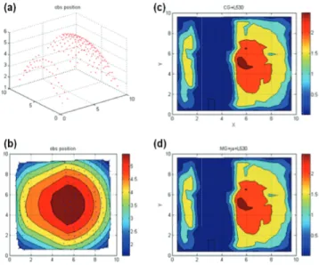
In the first idealized experiment, two dimensional (sur-face) temperature data fields were constructed, and the temperature data are plotted in Fig. 6 with randomly dis-tributed 179 surface temperature data items. The assump-tions for this experiment are as follows. The background error covariance B is a normal distribution, and the obser-vation error covariance R is an identity matrix. The given domain scale is 10km × 10km with a maximum grid level 4(16 × 16) and minimum grid level 2(4x4) and we use the V-cycle multigrid method. The observation operator is the composite of bi-linear interpolation and identity function.
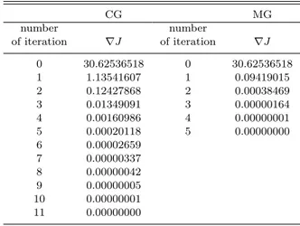
Under these conditions, we compare the iteration num-bers of the conjugate gradient method and that of the multigrid V-cycle with one pre-smoothing and one post-smoothing. For both algorithms, we stopped the iteration when the residual was less than 10−8. We see that the multi-grid (V-cycle) converges to the approximate solution with fewer iterations than the conjugate gradient method (Ta-ble 1). However, we see that the analysis fields of 3D-Var obtained by the multigrid method is just the same as the analysis fields obtained by the conjugate gradient method (Fig. 6).
4.2 Experiment 2
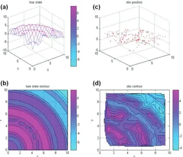
For the second experiment, again two dimensional (sur-face) temperature data fields were used as plotted in Fig. 7 with randomly distributed 179 surface temperature data items. In this experiment the data had more diverse wave-lengths than in the first experiment. The other conditions were the same as in the first experiment. Again, the multi-grid (V-cycle) converged to the approximate solution with fewer iterations than the conjugate gradient method (Table 2). We see that the analysis fields of 3D-Var by both methods are almost the same after the residual fell below the toler-ance (Fig. 8). However, there were differences in some areas during the iterations, see Fig. 8(a) and Fig. 8(d). The one V-cycle multigrid iteration already shows correct field on the right top corner where the data are sparsely observed while the conjugate gradient method needed seven iterations.
Now let us compare the performances of the meth-ods. The computation was performed on a window based notebook PC. No parallelization was used. Let us count the total computational costs. One iteration of the V-cycle multigrid algorithm requires one pre-smoothing, one matrix-vector multiplication, one post-smoothing, and two matrix-vector addition/subtraction. Finally, there is data transfer between grids. Altogether, it costs (roughly) three matrix-vector mul-tiplication, two vector addition/subtraction and data trans-fer between grids.
Each iteration of the CG method requires (roughly) one matrix-vector multiplication, four inner product of vectors, two addition/subtraction. A rough comparison shows one multigrid V-cycle takes about two to three iterations of the CG method. Our numerical experiment shows that the V-cycle multigrid takes four iterations while the CG takes ten to twelve iterations. Thus the total cost of the multigrid method seems comparable with that of CG. However, there is some room to improve the MG; for example, using dif-ferent smoothers or changing damping factors. There are also other variations, such as a W-cycle and FMV, which is known to be slightly better in practice. Still, a fair compar-ison would not be easy. It would be interesting if someone could implement the multigrid algorithm to solve real-life problems on parallel machines with various smoothers.
5 Conclusion
In this study, we introduced the multigrid method for the minimization process in data assimilation by interpret-ing the minimization process as a numerical PDE discretized by the CCFD. We designed the prolongation and restriction operators based on this observation. We performed some numerical experiments and compared them with the con-jugate gradient method. We see that the multigrid method has fewer iterations than the conjugate gradient method and converges faster on the data-sparse area. A generalization of our multigrid algorithm for other data such as wind field in three dimensional space is left for our future research.
6 Acknowledgments
We would like to thank the anonymous referees who gave many helpful comments to improve the quality of the
manuscript. This work partially supported by the Korea Me-teorological Administration.
REFERENCES
Baker, D.M., Huang, Wei, Guo, Y.-R, and A., Bourgeois, 2003. A three-dimensional variational(3DVAR) data assimilation system for use with MM5. NCAR Tech. Note 453, 68. Baker, D.M., Huang, Y.-R., Guo, A., Bourgeois, and, Xiao, Q.,
2003. A three-dimensional variational data assimilation sys-tem for use with MM5: Implementation and initial results. Mon. Wea. Rev 132, 897–914.
F. Bouttier, and P. Courtier, 2002. Data assimilation concepts and methods. ECNWF, Meteorological Training Course Lec-ture Seriese. 117, 279–285.
J. H. Bramble, R. Ewing, J. E. Pasciak, and J. Shen, 1996. The Analysis of Multigrid Algorithms for Cell Centered Finite Difference Methods. Adv.Compute.Math. 5, 1–34.
Briggs, William L., Henson, V. E., and McCormick, S. F., 2000. A multigrid tutorial. 2nd ed. SIAM.
Downton, R. A.,and Bell, R.S., 1998. The impact of analysis dif-ferences in a medium-range forecast. Meteorol. Mag. 117, 279–285.
Gratton S., Tointc P. L.,Tshimangaa J., 2013. Conjugate gradi-ents versus multigrid solvers for diffusion-based correlation models in data assimilation Q. J. Royal Meteoro. Soc. 139 1481–1487.
Kwak, Do Y., 1999. V-cycle multigrid for cell-centered finite dif-ferences. SIAM J. Scientific Computing 21 no 2, 552–564. Li, Wei, Xie, Yuanfu, Deng, Shiow-Ming, and Wang, Qi, 2010.
Ap-plication of the Multigrid Method to the Two-Dimensional Doppler Radar Radial Velocity Data Assimilation. J. Atmos. Oceanic Technol. 27, 319–332.
Li, Wei, Xie, Yuanfu, He, Zhongjie, Han, Guijun,Liu, Kexiu, and Li, Dong, 2008. Application of the Multigrid Data Assimi-lation Scheme to the China Seas Temperature Forecast. J. Atmos. Oceanic Technol. 25, 2106–2116.
Richardson, D., 1998. The relative effect of model and analysis differences on ECMWF and UKMO operational forecasts. In Proceedings of the ECMWF workshop on predictability, ECMWF, Shinfield Park, Reading, UK(20-22 October 1997). Zou, Xiaolei, Vandenberghe, F., Pondeca, M. and Kuo, Y.-H. 1997. Introduction to adjoint techniques and the MM5 ad-joint modeling system. NCAR Technical Note.
Xiao, Q. Kuo,Y.-H., Sun,J.. Lee, W.-C., Barker, D.M. and Lim, E.,2007. An approach of radar reflectivity data assimila-tion and its assessment with the island QPF of Typhoon Rusa(2002) at landfall. J. Appl. Meteor. Climatol. 46, 14– 22.
Xiao, Q. Lim, E., Won, D.-J., Sun, J., Lee, C., M.-S. Lee, W.-J. Lee, W.-J.-Y. Cho,Y.-H. Kuo, D. Barker, D., Lee, D.-K., and Lee, H.-S., 2008. Doppler radar data assimilation in KMA’s operational forecasting. Bull., Amer. Meteor. Soc. 89, 39– 43.
Xie, Y., Koch, S. McGinley, J. and Albers, S., Bieringer,P. E., Wolfson, M., Chan, M., 2010. A Space-Time Multiscale Anal-ysis System: A Sequential Variational AnalAnal-ysis approach. AMS. Monthly Weather. Review 139, 1124–1240.
Table 1. The result of numerical experiment 1. CG MG number number of iteration ∇J of iteration ∇J 0 30.62536518 0 30.62536518 1 1.13541607 1 0.09419015 2 0.12427868 2 0.00038469 3 0.01349091 3 0.00000164 4 0.00160986 4 0.00000001 5 0.00020118 5 0.00000000 6 0.00002659 7 0.00000337 8 0.00000042 9 0.00000005 10 0.00000001 11 0.00000000
Table 2. The result of numerical experiment 2.
CG MG number number of iteration ∇J of iteration ∇J 0 20.43552705 0 20.43552705 1 2.64095750 1 0.06380830 2 0.41885882 2 0.00026161 3 0.06872520 3 0.00000117 4 0.01019913 4 0.00000001 5 0.00176452 5 0.00000000 6 0.00031169 7 0.00005252 8 0.00000787 9 0.00000138 10 0.00000020 11 0.00000003 12 0.00000001 13 0.00000000
Figure 1. The smoothing property
Figure 2. Schedule of grids for (a) V-cycle, (b)W-cycle, (3) FMV-cycle.
Figure 3. The minimization procedure of the Incremental 3D-Var
Figure 4. The horizontal grid structures of WRF (a) WRF model : Arakawa C-grid staggering, (b) WRF-Var : unstaggered Arakawa A-grid
Figure 5. (a) non-weighted prolongation for CCFD, (b) weighted prolongation for CCFD
Figure 6. (a) The observation data, (b) The contour of obser-vation data, (c) The analysis field of 3D-Var with the conjugate gradient method, (d) The analysis field of 3D-Var with the multi-grid method.
Figure 7. (a) The true state of temperature, (b) The contour of true data, (c) The observation data (b) The contour of observa-tion data.
Figure 8. (a)-(c) : The analysis fields of 3D-Var with the conju-gate gradient method at each iterative step 1(a), 7(b), and 13(c), (d)-(f): The analysis fields of 3D-Var with the multigrid method at each iterative step 1(d), 3(e), and 5(f).